Chapter 2

2.1 The Basic Muskingum Flood Routing Method

Typically, the inflow hydrograph used in flood routing is derived by converting a measured stage into discharge using a steady state rating curve (Mutreja, 1986; Perumal and Raju, 1998; Moramarco and Singh, 2001).

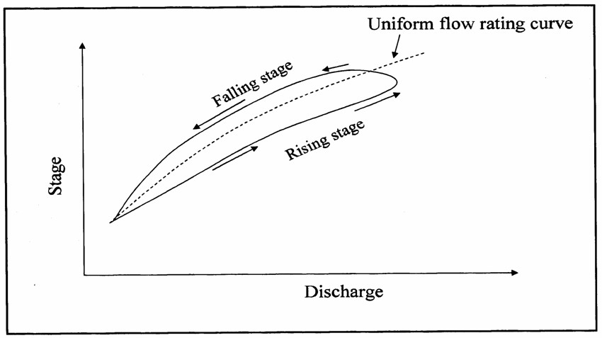
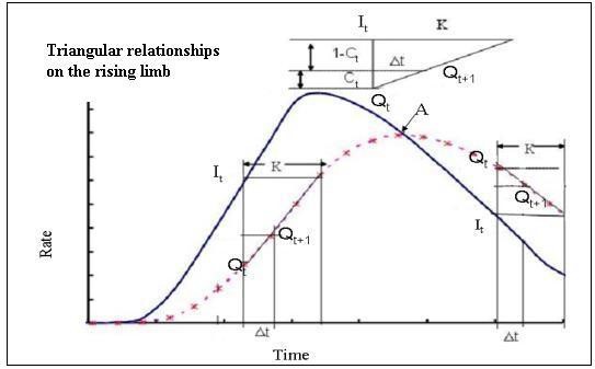
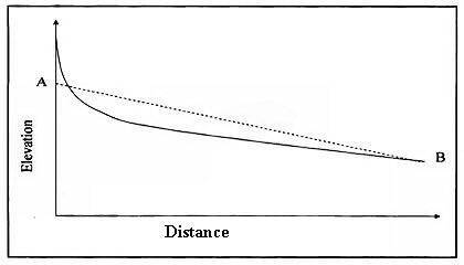
As illustrated by Shaw (1994), storage in a river reach can be categorized into three forms, as depicted in Figure 2.1. During the rising stage of a flood in the reach, when inflow exceeds outflow, wedge storage must be added to prism storage. Conversely, during the falling stage, when inflow is less than outflow, wedge storage is negative and subtracted from prism storage to calculate total temporary storage in the reach. When outflow and inflow are equal in a reach, only prism storage is present in the channel.

Figure 2.1 Storage and non-steady flow (after Shaw, 1994).

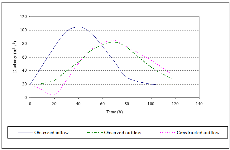
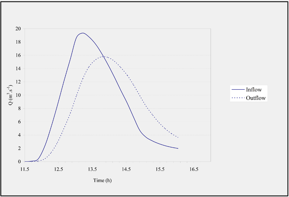
Figure 2.2 illustrates an example of inflow and outflow hydrographs to and from a reach with prism storage. In a river reach characterized by a uniform cross-section and constant slope, velocity remains unchanged, indicating uniform flow (Chow, 1959). In these reaches, the peak of the outflow hydrograph aligns with the recession curve of the inflow hydrograph (Shaw, 1994).

Figure 2.2 Example of inflow and outflow hydrographs.

According to Tung (1985) and Fread (1993), the most common form of the linear Muskingum model is expressed as the following equations:

S_p = KQ_t (2.1)

S_w = K(I_t - Q_t)X (2.2)

where

S_p	temporary prism storage [m³]
S_w	temporary wedge storage [m³]
I_t	the rate of inflow [m³/s] at time t
Q_t	outflow [m³/s] at time t
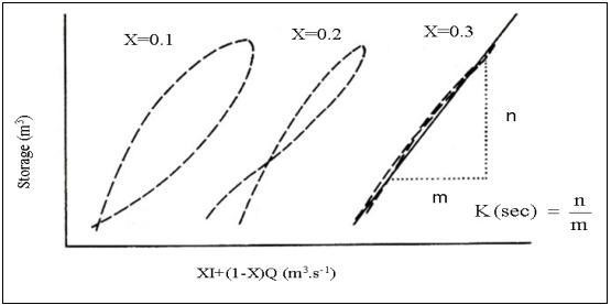
K	the storage time constant for the river reach, with a value close to the wave travel time within the river reach [s]
X	a weighting factor varying between 0 and 0.5 [dimensionless]

By combining Equations 2.1 and 2.2, the basic Muskingum equation is attained as given in Equations 2.3a and 2.3b:

S_t = S_p + S_w (2.3a)

S_t = K[XI_t + (1 - X)Q_t] (2.3b)

where

S_t	temporary channel storage [m³] at time t
S_p	prism storage at time t
S_w	wedge storage at time t

When X = 0, Equation 2.3 simplifies to S_t = KQ_t, indicating that storage is solely dependent on outflow. When X = 0.5, equal weight is given to inflow and outflow, resulting in a condition akin to a uniformly progressive wave that does not attenuate (US Army Corps of Engineers, 1994a). Thus, 0.0 and 0.5 serve as limits for the value of X, determining the degree of attenuation of a flood wave within this range as it passes through the routing reach (US Army Corps of Engineers, 1994a).

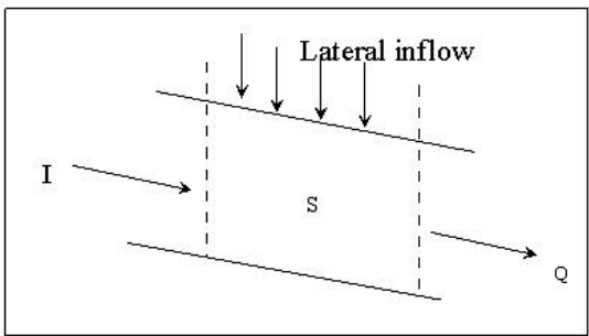
Fread (1993) explained that an oversimplified depiction of unsteady flow along a routing reach may be seen as a lumped process, wherein the inflow at the upstream end and the outflow at the downstream end of the reach vary with time. In Muskingum flood routing, it is assumed that the storage in the system at any moment is proportionate to a weighted average of inflow and outflow from a given reach (Bauer, 1975).

According to the continuity equation (Equation 2.4), the rate of change of storage in a channel over time equals the difference between inflow and outflow (Shaw, 1994):

ΔS_t/Δt = I_t - Q_t (2.4)

where

ΔS_t/Δt	the rate of change of channel storage with respect to time

The combination and solution of Equations 2.3 and 2.4 in finite difference form yield the well-known Muskingum flow routing equations as presented in Equations 2.5 and 2.6.

Q_j+1^t+1 = C₀I_j^t + C₁I_j^t+1 + C₂Q_j+1^t (2.5)

where

Q_j^t	outflow at time t of the j^th sub-reach
I_j^t	inflow at time t of the j^th sub-reach

C₀ = (Δt + 2KX)/m (2.6a)

C₁ = (Δt - 2KX)/m (2.6b)

C₂ = (2K(1 - X) - Δt)/m (2.6c)

m = 2K(1 - X) + Δt (2.6d)

Here, C₀, C₁, and C₂ represent coefficients determined by functions of K, X, and a discretized time interval Δt. The sum of C₀, C₁, and C₂ equals one, so once C₀ and C₁ are calculated, C₂ can be derived as 1 - C₀ - C₁. Consequently, the outflow at the end of a time step is the weighted sum of the initial inflow and outflow, as well as the final inflow (Shaw, 1994). These three coefficients remain constant throughout the routing process (Fread, 1993).

As suggested by Viessman et al. (1989), it is important to avoid negative values for C₁. This is ensured when Equation 2.7 is satisfied. Negative values of C₂, however, do not impact the hydrographs routed during flooding (Viessman et al., 1989).

Δt / K > 2X (2.7)

Figure 2.3 Cunge curve (Cunge, 1969 cited by NERC, 1975).

The time Δt is called the routing period and it must be chosen sufficiently small such that the assumption of flow rate linearity over time interval Δt is approximated (Gill, 1992). In particular, if Δt is too large, the peak of the inflow curve may be missed, so the period should be kept smaller than 1/5 of the travel time of the flood peak through the reach (Wilson, 1990). According to Viessman et al. (1989), theoretical stability of the numerical method is accomplished if Equation 2.8 is fulfilled:

2KX ≤ Δt ≤ 2K(1 - X) (2.8)

Figure 2.4 River routing storage loops (after Wilson, 1990).

Figure 2.5 Muskingum routed hydrographs (after Shaw, 1994).

Figure 2.6 Loop-rating curve (after NERC, 1975).

2.2 The Muskingum-Cunge Parameter Estimation Method with Lateral Inflow

The original Muskingum method is based on the storage equation with the coefficients K and X derived by trial and error. Unlike the basic Muskingum method where the parameters are calibrated based on observed stream flow data, in the Muskingum-Cunge method parameters are calculated based on flow and channel characteristics. Hence, in the absence of observed flow data, the Muskingum-Cunge method may be used for parameter estimation.

K = ΔL / V_w (2.9)

X = (1/2) - Q₀ / 2SWV_wΔL (2.10)

As seen in Equations 2.9 and 2.10, the Muskingum-Cunge K and X parameters are obtained using variables such as the top width of the river, wave celerity, reach cross-section area, reach length, and reach slope. The relation of the Muskingum K and X parameters to catchment characteristics makes the Muskingum-Cunge method suitable for application to ungauged streams.

Q₀ = Q_b + 0.5(Q_p - Q_b) (2.11)

V_w = ΔQ / ΔA (2.12)

Q_j+1^t+1 = C₀I_j^t + C₁I_j^t+1 + C₂Q_j+1^t + C₃ (2.13)

C₃ = (q*Δt*ΔL / 2K(1-X)) + Δt (2.14)

The Saint-Venant Equation for gradually varying flow in open channels is given as follows:

q = ΔA / Δt + ΔQ / ΔL (2.15a)

ΔA / Δt ≅ ((A_j^t+1 + A_j+1^t+1)/2 - (A_j^t + A_j+1^t)/2)/Δt (2.15b)

ΔQ / ΔL ≅ (β(Q_j+1^t+1 - I_j^t+1) + (1-β)(Q_j+1^t - I_j^t))/ΔL (2.15c)

Δt ≥ 1.625µ/V_w and 2.6µ/V_w ≤ ΔL ≤ 1.6V_wΔt (2.16a)

μ = Q₀ / (2WS)

ΔL ≅ 0.5V_wΔt [1 + (1 + 1.5Q₀/(V_w²SΔt))^1/2] (2.16b)

2.3 The Three-parameter Muskingum Procedure with Lateral Inflow

The Three-parameter Muskingum procedure is a method based on the three-parameter Muskingum model, where the two conventional parameters are augmented by a third parameter to account for lateral inflow into the reach.

Figure 2.7 Lateral inflow model (after O'Donnell et al., 1988).

I_t(1 + α) = Q_t + dS/dt (2.17)

S_t = K[X(1 + α)I_t + (1 - X)Q_t] (2.18)

|Q_(t+1)| = |I_t, I_(t+1), Q_t| * |d_i| (2.19)

2.4 Application of the Three-parameter Muskingum Model (Matrix)

In a study conducted on two British rivers, the Wye and the Wyre, O'Donnell et al. (1988) demonstrated the dependency of the α parameter on individual flood events and recommended further studies to investigate α values in relation to storm rainfall distribution.

2.5 The Non-linear Muskingum Method

It is recognised that the storage versus weighted flow relationship is not always linear as is implied in Equation 2.3. If the relationship is non-linear, use of Equation 2.3 introduces considerable error.

S = K[XI_t + (1 - X)Q_t]ⁿ (2.23)

S = K[XI_t^m + (1 - X)Q_t^m] (2.24)

2.6 The SCS Convex Method

The US Soil Conservation Service developed a coefficient channel routing technique similar to the Muskingum method. It has had widespread use in project planning and is used successfully even when limited storage data for the reach is available.

If I_t ≥ Q_t, then I_t ≥ Q_t+1 ≥ Q_t (2.25)

If I_t ≤ Q_t, then I_t ≤ Q_t+1 ≤ Q_t (2.26)

Q_t+1 = Q_t + C_t(I_t - Q_t) (2.27)

C_t = (Q_t+1 - Q_t)/(I_t - Q_t) (2.28)

Figure 2.8 Channel routing using the Convex method (after NRCS, 1972).

2.7 Discharge and Channel Relationships

As suggested by Clark and Davies (1988), rivers have a unique relationship between flow and channel dimensions, although close similarities are found for rivers in the same region with similar bed and bank materials and similar sediment loads.

b = zQ^m (2.29)

Table 2.1 Coefficients of Equation 2.29 (after Clark and Davies, 1988).

References	z	m
Nixon (1959)	2.99	0.50
Simons and Albertson (1963)	2.85	0.50
Kellerhals (1976)	3.26	0.50
Charlton et al. (1979)	3.74	0.45
Bray (1982)	4.75	0.53
Hey and Thorne (1987)	3.67	0.45

2.8 Flood Routing in Ungauged Rivers

The Muskingum-Cunge routing model uses channel geometry, reach length, roughness coefficient, and slope to estimate the parameters of the model. Therefore, the Muskingum-Cunge method may be used for flood routing analysis in an ungauged catchment.

2.9 Factors that Influence Flood Routing

The factors influencing the practical application of the Muskingum flood routing method should be considered in parameter estimation techniques.

2.9.1 Slope

Fr = V_av / √(gc) (2.34)

Figure 2.9 Mean stream slope (after Linsley et al., 1988).

2.9.2 Backwater and inundation effects

Hydrological flood routing methods typically overlook variable backwater effects, such as downstream dams, constrictions, bridges, and tidal influences.

2.9.3 Manning roughness coefficient

Roughness coefficients indicate the resistance to flood flows within channels and floodplains.

Chapter Video

Muskingum Channel Routing Methods

2.1 The Basic Muskingum Flood Routing Method

2.2 The Muskingum-Cunge Parameter Estimation Method with Lateral Inflow

2.3 The Three-parameter Muskingum Procedure with Lateral Inflow

2.4 Application of the Three-parameter Muskingum Model (Matrix)

2.5 The Non-linear Muskingum Method

2.6 The SCS Convex Method

2.7 Discharge and Channel Relationships

2.8 Flood Routing in Ungauged Rivers

2.9 Factors that Influence Flood Routing

Information Box