5. RESULTS

Toggle Video

The results of applying the methodology outlined in Chapter 4 are contained in this chapter and include both results using calibrated parameters, to assess the performance of the Muskingum method, and results from using the Muskingum-Cunge method, to assess the performance of the method in ungauged catchments.

5.1 Flood Routing Using Observed Inflow  and Outflow Hydrographs

Flood routing using calibrated parameters was undertaken and events that had good inflow and outflow hydrographs were considered for further sensitivity analysis. Single observed events were extracted from each sub-catchment, as detailed in Section 4.3. The extracted hydrographs were analysed using the M-Cal and M-Ma parameter estimation methods. The details of the results and plotted hydrographs are contained in the following sub-sections.

5.1.1 Reach-I

The estimated catchment characteristics and parameters for Reach-I are contained in Tables 5.1 to 5.3.

Table 5.1 Estimated parameters for Reach-I using the M-Cal method.

Reach	Event	ΔL [m]	Δt [s]	A [m2]	Q0 [m3/s]	K [s]	X	C0	C1	C2
I	1	2045	1800	65.90	61.26	1800	0	0.33	0.33	0.33
	2	2045	2520	82.21	54.58	2520	0	0.33	0.33	0.33
	3	4090	1800	35.73	66.43	1800	0	0.33	0.33	0.33

Table 5.2 Estimated parameters for Reach-I using the M-Ma method.

Reach	Event	ΔL [m]	Δt [s]	A [m2]	Q0 [m3/s]	K [s]	X	C0	C1	C2	α
I	1	4090	1800	65.90	61.26	4895	-0.26	-0.06	0.31	0.75	-0.07
	2	4090	2520	82.21	54.58	3700	-0.02	0.23	0.27	0.50	-0.12
	3	4090	1800	35.73	66.43	2748	-0.33	0.00	0.40	0.60	-0.03

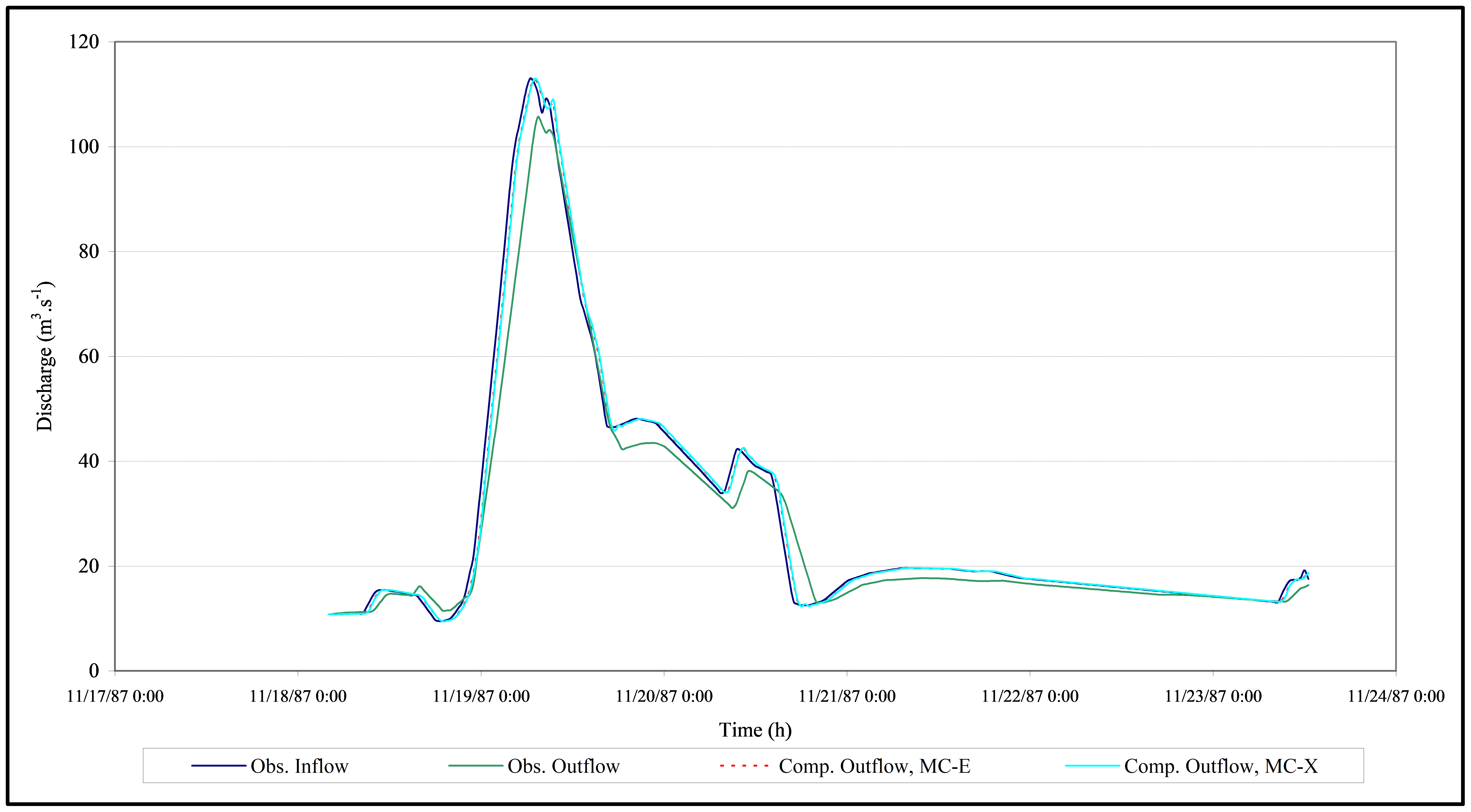
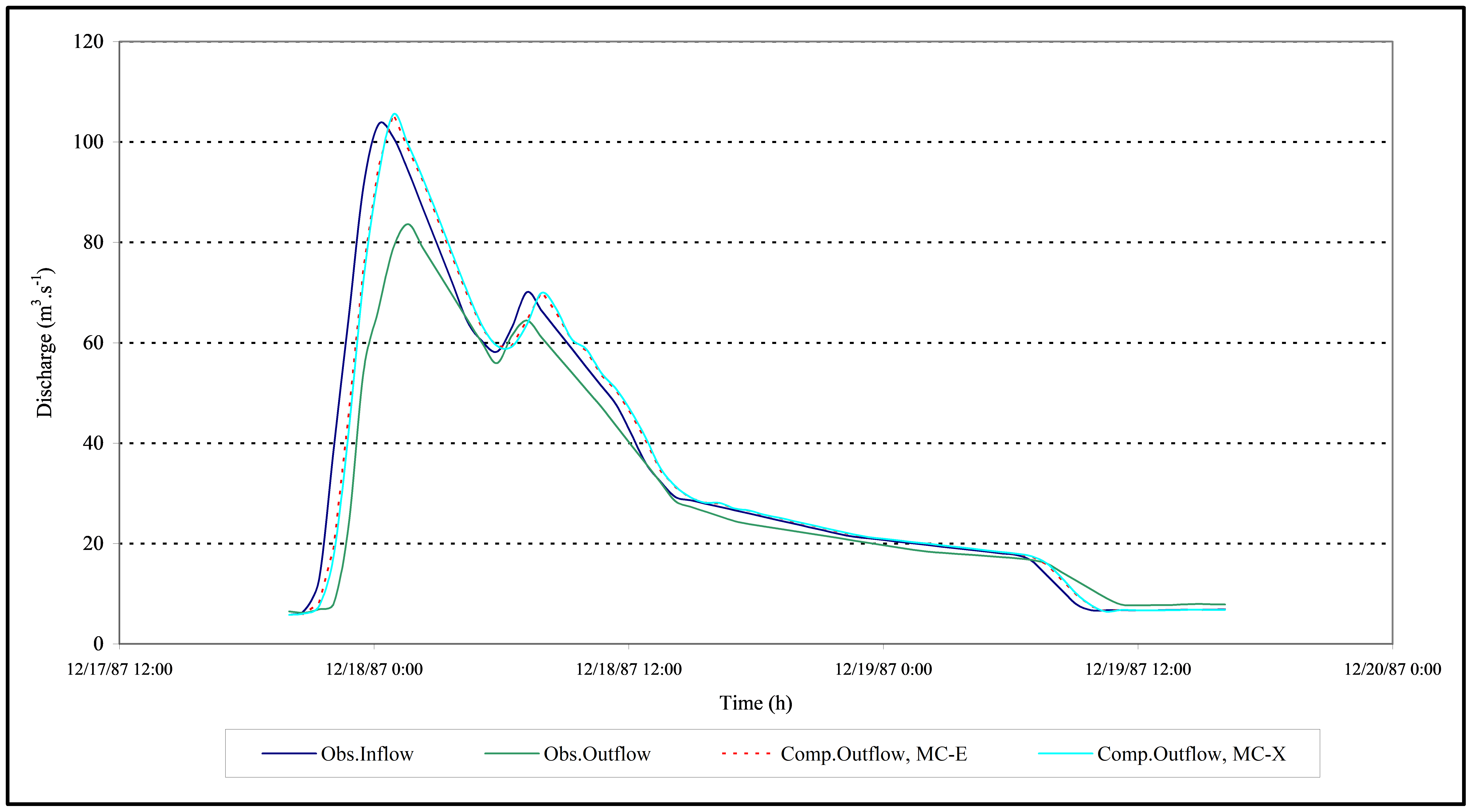
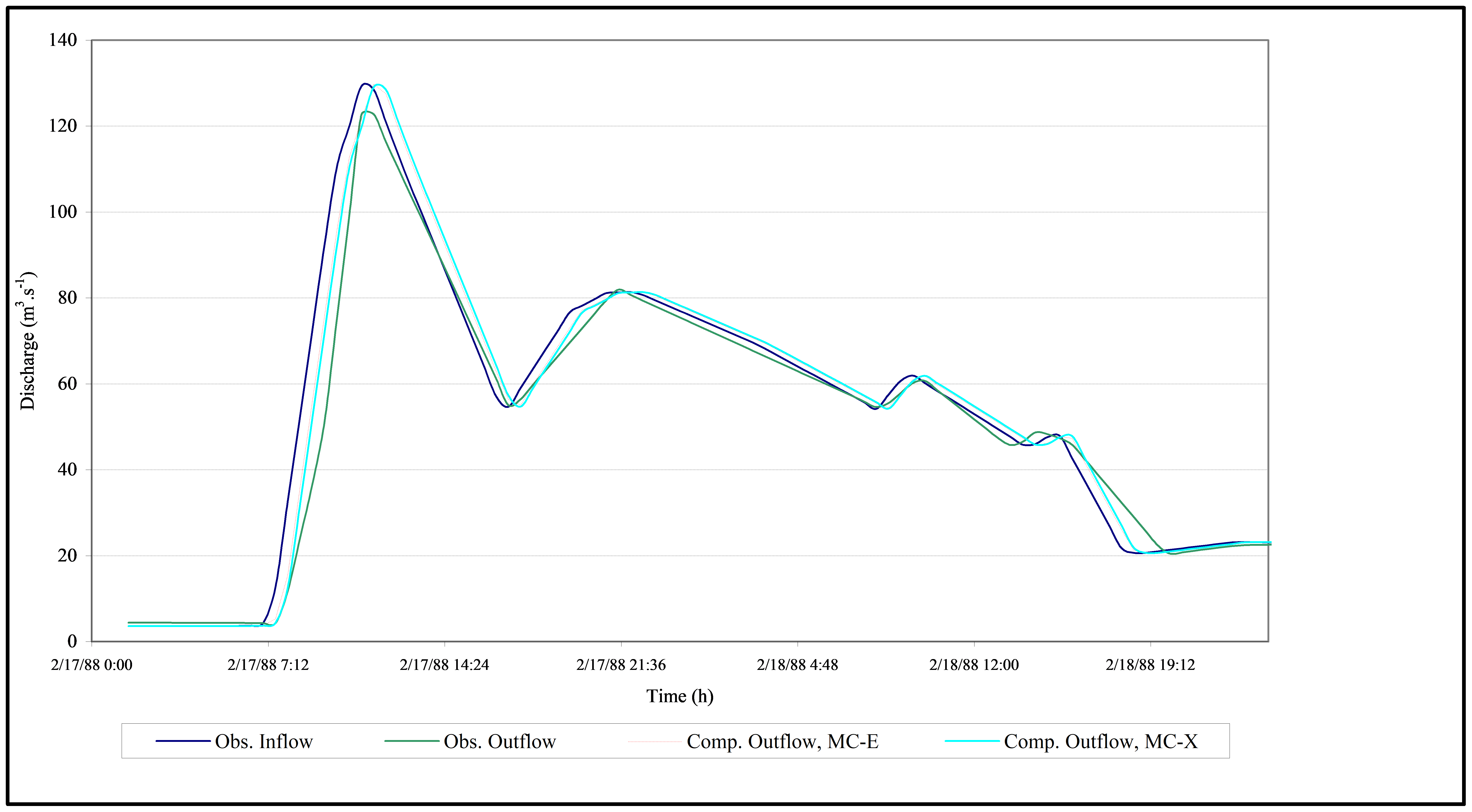
The computed and observed hydrographs from the application of the M-Cal and M-Ma methods for events in Reach-I are shown in Figures 5.1 to 5.3.

The results from using the M-Cal and M-Ma parameter estimation methods for Reach-I are contained in Tables 5.3 to 5.4.

Table 5.3 Results for Reach-I using the M-Cal method.

Reach	Events	Obs Peak flow [m3/s]	Comp Peak flow [m3/s]	Peak flow Error [%]	Peak timing Error [%]	RMSE [m3/s]	Coefficient of efficiency (E)	Obs Volume [million cubic meters]	Comp Volume [million cubic meters]	Volume Error [%]
I	1	105.70	111.07	5.08	-1.59	3.34	0.98	12.63	13.44	6.44
	2	83.67	94.27	12.67	-5.47	6.42	0.92	4.88	5.49	12.58
	3	122.79	125.54	2.24	-5.00	3.80	0.98	10.72	11.00	2.61

Table 5.4 Results for Reach-I using the M-Ma method.

Reach	Events	Obs Peak outflow [m3/s]	Comp Peak Outflow [m3/s]	Peak flow Error [%]	Peak timing Error [%]	RMSE [m3/s]	Coefficient of efficiency (E)	Obs Volume [million cubic meters]	Comp Volume [million cubic meters]	Volume Error [%]
I	1	103.20	100.00	-3.10	1.59	1.69	0.99	12.63	12.57	0.52
	2	83.60	82.33	-1.52	0.00	2.37	1.00	4.88	4.84	0.81
	3	122.40	114.79	-6.22	0.00	2.97	0.99	10.72	10.62	0.96

From the analyses of events using the M-Cal and the M-Ma method shown in Tables 5.1 to 5.4, it is noted that the methods have different K and X values. The K parameter in the M-Cal and the M-Ma methods are different. The K parameters from the M-Ma method are for the whole reach, but the K parameters from the M-Cal method are for the sub-routing reaches (ΔL). The X values are negative in the M-Ma method. As noted by O'Donnell et al. (1988), the calibration procedure requires many events to be analysed to define the most appropriate X value for the selected reach. Since the M-Ma method cannot be applied in ungauged catchments as it requires observed inflow and outflow hydrographs, it is not necessary to analyse many events for the assessment of M-Ma method in the present study.

From the results for the M-Cal method for Reach-I, contained in Table 5.3, the computed peak outflow is larger than the observed peak discharge for all three events considered. This may be explained by the fact that the M-Cal equation does not consider any lateral outflows which might happen due to infiltration and activities such as irrigation or diversion for other purposes. Additionally, incorrect estimation of the slope may have contributed to these discrepancies, which in turn affected the computation of the outflow hydrographs.

The negative α value shown in Table 5.2 indicates that there is no lateral inflow but that there are outflows from the main reach. Despite this, both methods exhibit small RMSE values and 'E' values that are nearly equal to 1, suggesting a small error in the computed hydrographs and a similar shape between the observed and computed hydrographs.

The computed outflow hydrographs generated by the M-Ma method (Table 5.4 and Figure 5.1) closely resemble the observed outflow hydrograph, with the exception of slightly lower peaks observed in Events 1 and 3. This discrepancy may be attributed to the direct calibration of parameters from the inflow and observed outflow hydrographs in the M-Ma method.

Although the K and X parameters differ between the M-Cal and M-Ma methods, the computed hydrographs exhibit similar characteristics to the observed hydrograph, including peak flow, peak flow time, volumes, and overall shape. However, negative values for peak flow error, peak timing error, and volume error indicate that the computed results are generally smaller than the observed values. Despite these differences, the RMSE values obtained from the analyses suggest that the errors are relatively small. It's worth noting that an X value of 0.0 in the M-Cal method implies that storage is solely a function of outflow.

Based on the results from both methods, it can be concluded that the Muskingum method, with calibrated parameters, produces computed hydrographs in Reach-I that closely resemble the observed hydrographs in terms of volume and shape. Comparing the two methods, the M-Ma method exhibited slightly better performance than the M-Cal method, as indicated by the E and volume error statistics.

5.1.2 Reach-II

The catchment characteristics and parameters estimated for Reach-II are contained in Tables 5.5 to 5.8.

Table 5.5 Estimated parameters for Reach-II using the M-Cal method.

Reach	Event	ΔL [m]	Δt [s]	A [m2]	Q0 [m3/s]	K [s]	X	C0	C1	C2
II	1	7777	5400	23.18	27.32	5400	0.49	0.98	0.01	0.01
	2	7777	5400	26.64	31.39	5400	0.49	0.98	0.01	0.01
	3	7777	5400	20.50	30.26	5400	0.49	0.98	0.01	0.01
	4	7777	5400	22.10	26.04	5400	0.49	0.98	0.01	0.01

Table 5.6 Estimated parameters for Reach-II using the M-Ma method.

Reach	Event	ΔL [m]	Δt [s]	A [m2]	Q0 [m3/s]	K [s]	X	C0	C1	C2	α
II	1	54440	5400	23.18	27.32	59090	0.16	0.23	-0.13	0.90	0.20
	2	54440	5400	26.64	31.39	99491	0.23	0.32	-0.25	0.93	0.04
	3	54440	5400	20.50	30.26	32400	-0.37	-0.20	0.31	0.89	0.20
	4	54440	5400	22.10	26.04	9200	-4.09	-0.71	0.81	0.89	-0.06

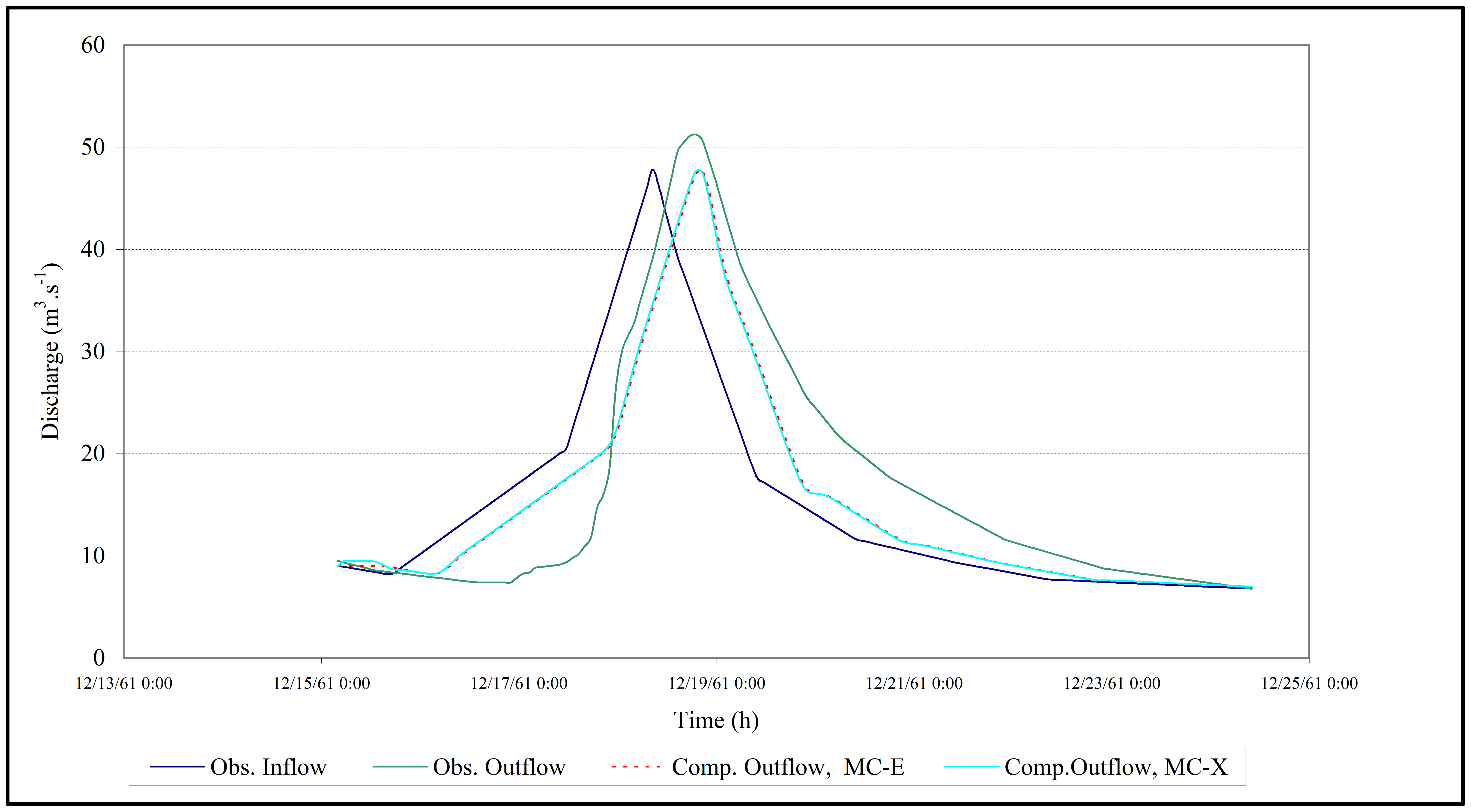
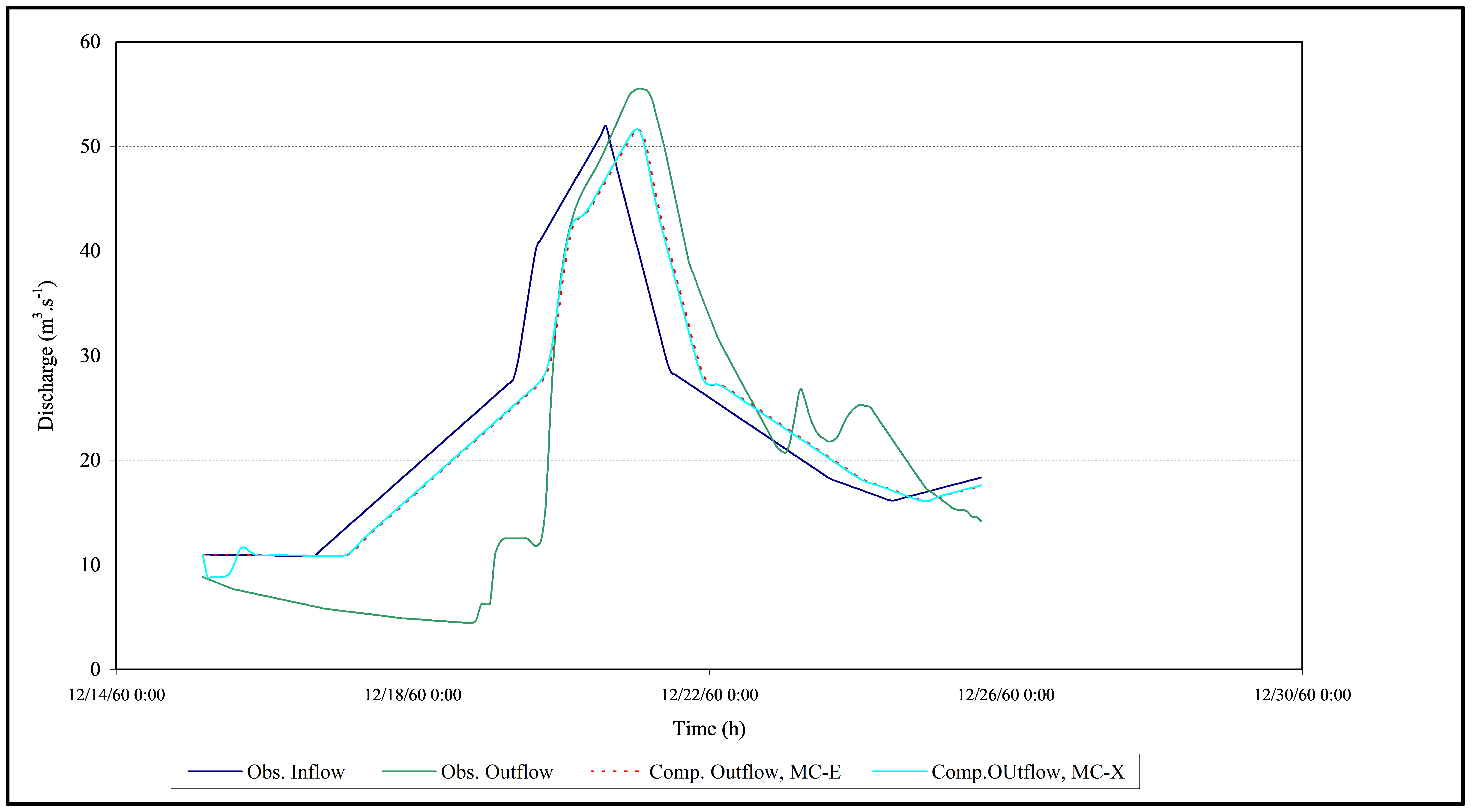
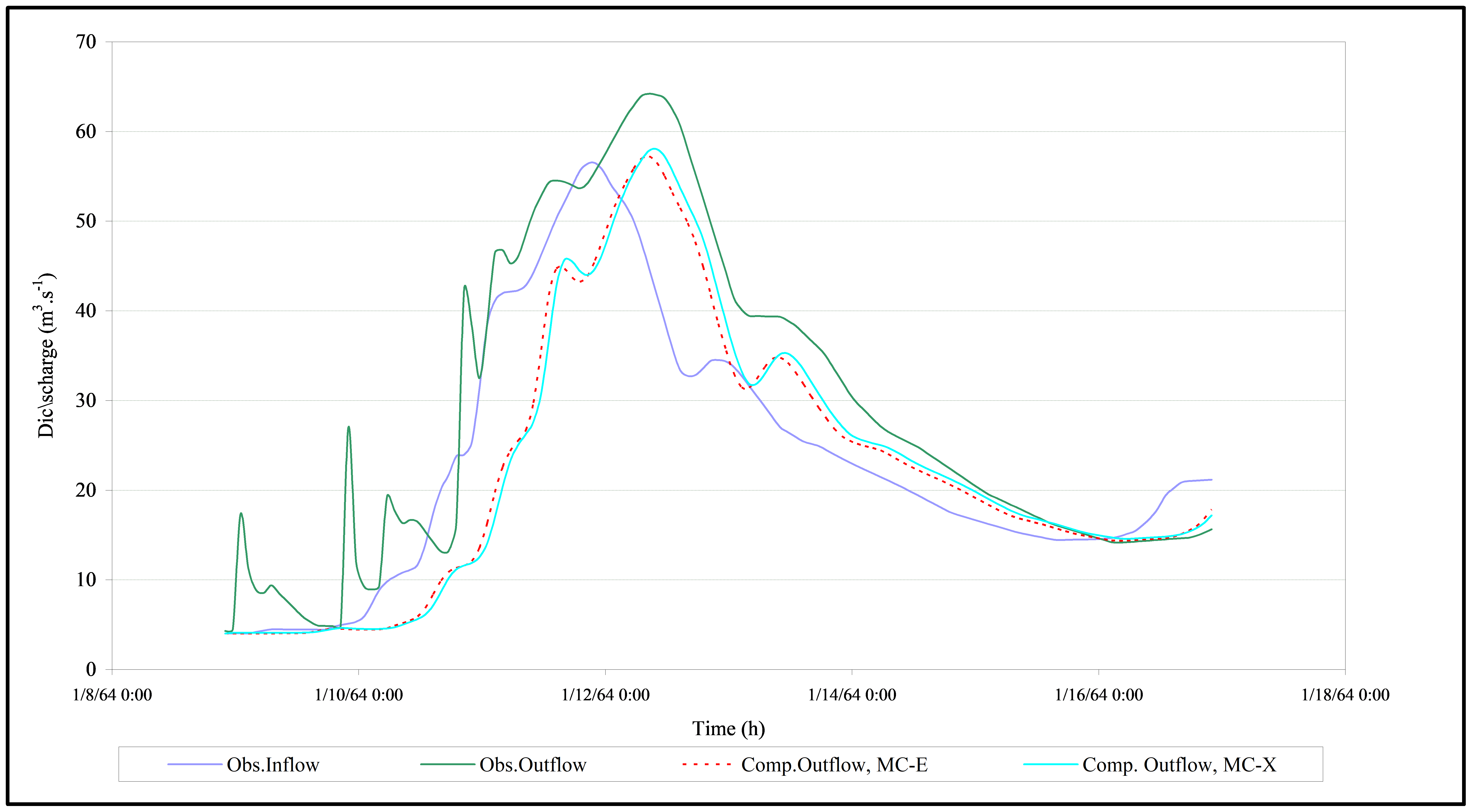
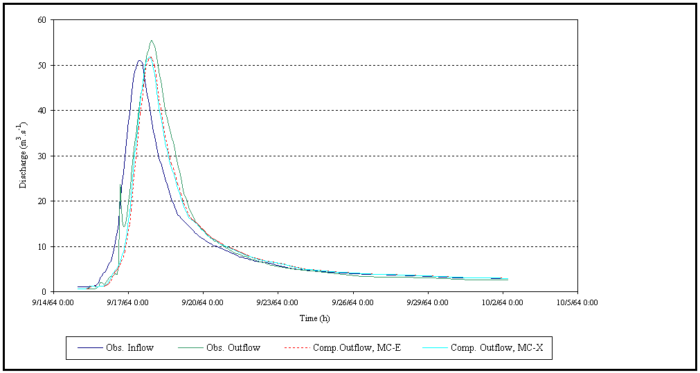
The computed and observed hydrographs for events in Reach-II using both the M-Cal and the M-Ma method are shown in Figures 5.4 to 5.7.

The results of flood routing analyses for Reach-II using the M-Cal method and the M-Ma method are contained in Tables 5.7 and 5.8.

Table 5.7 Results for Reach-II using the M-Cal method.

Reach	Event	Obs Peak outflow m3/s]	Comp Peak outflow [m3/s]	Peak flow Error [%]	Peak timing Error [%]	RMSE [m3/s]	Coefficient of efficiency (E)	Obs Volume [million cubic meters]	Comp Volume [million cubic meters]	Volume Error [%]
II	1	51.25	47.98	-6.38	3.30	4.39	0.88	13.63	12.39	-9.08
	2	55.52	51.85	-6.61	1.03	7.07	0.83	18.54	20.57	10.96
	3	64.22	55.53	-13.53	-2.87	10.50	0.65	19.87	15.45	-22.24
	4	55.40	51.87	-6.36	1.60	2.24	0.97	14.39	13.74	-4.52

Table 5.8 Results for Reach-II using the M-Ma method.

Reach	Event	Obs Peak outflow [m3/s]	Comp Peak [m3/s]	Peak flow Error [%]	Peak timing Error [%]	RMSE [m3/s]	Coefficient of efficiency (E)	Obs Volume [million cubic meters]	Comp Volume [million cubic meters]	Volume Error [%]
II	1	51.25	44.67	-12.83	0.00	3.66	0.91	13.63	14.85	8.97
	2	55.52	44.85	-19.23	1.03	1.56	0.99	18.54	20.95	13.01
	3	64.22	58.96	-8.19	0.00	5.93	0.89	19.87	18.89	-4.92
	4	55.40	44.86	-19.03	1.60	5.14	0.84	14.39	12.91	-10.24

In Reach-II, lateral inflow occurs due to the length of the reach. Therefore, the computation of the hydrographs includes the addition of lateral inflow into the main stream.

The volume errors exceed 5% for Events 1, 2, and 3 using the M-Cal method, and for Events 1, 2, and 4 using the M-Ma method. Despite this, upon examination of the hydrographs, RMSE, and E values, it becomes apparent that the shape of the computed hydrographs closely resembles that of the observed outflow hydrographs for both methods.

While the K and X parameters differ between the two methods, the computed hydrographs closely resemble the observed outflow hydrographs in terms of peak flow, peak flow time, volume, and overall shape. The value of X = 0.49 suggests an equal weighting between inflow and outflow hydrographs in the routing procedure.

5.1.3 Reach-III

The estimated catchment characteristics and parameters for Reach–III are contained in Tables 5.9 and 5.10.

Table 5.9 Estimated parameters for Reach-III using the M-Cal method.

Reach	Event	ΔL [m]	Δt [s]	A [m2]	Q0 [m3/s]	K [s]	X	C0	C1	C2
III	1	4000	9000	50.85	18.49	9000	0.49	0.98	0.01	0.01
	2	4000	9000	43.40	26.31	9000	0.49	0.98	0.01	0.01
	3	10000	9000	24.30	22.09	9000	0.50	1.00	0.00	0.00
	4	10000	9000	13.08	11.89	9000	0.39	0.80	0.10	0.10

Table 5.10 Estimated parameters for Reach-III using the M-Ma method.

Reach	Event	ΔL [m]	Δt [s]	A [m2]	Q0 [m3/s]	K [s]	X	C0	C1	C2	α
III	1	20000	9000	50.85	18.49	54624	0.12	0.22	-0.04	0.83	0.09
	2	20000	9000	43.40	26.31	52914	0.35	0.60	-0.36	0.77	0.00
	3	20000	9000	24.30	22.09	18574	0.53	1.09	-0.41	0.32	-0.05
	4	20000	9000	13.08	11.89	26257	0.43	0.81	-0.34	0.54	-0.09

The computed and observed hydrographs for events in Reach-III using both the M-Cal and the M-Ma method are shown in Figures 5.8 to 5.11.

The results of flood routing analysis using the M-Cal and M-Ma methods in Reach-III are contained in Tables 5.11 and 5.12 following.

Table 5.11 Results for Reach-III using the M-Cal method.

Reach	Event	Obs Peak outflow [m3/s]	Comp Peak outflow [m3/s]	Peak flow Error [%]	Peak timing Error [%]	RMSE [m3/s]	Coefficient of efficiency (E)	Obs Volume [million cubic meters]	Comp Volume [million cubic meters]	Volume Error [%]
III	1	40.65	39.40	-3.07	2.38	2.75	0.90	10.34	9.62	-6.97
	2	52.97	43.74	-17.41	0.00	4.14	0.82	11.08	11.56	4.36
	3	39.64	39.54	-0.27	0.00	1.69	0.96	8.72	9.45	8.37
	4	19.97	19.92	-0.26	0.00	0.99	0.91	5.67	6.36	12.31

Table 5.12 Results for Reach-III using the M-Ma method.

Reach	Event	Obs Peak outflow [m3/s]	Comp Peak [m3/s]	Peak flow Error [%]	Peak timing Error [%]	RMSE [m3/s]	Coefficient of efficiency (E)	Obs Volume [million cubic meters]	Comp Volume [million cubic meters]	Volume Error [%]
III	1	40.65	29.61	-27.15	2.38	2.97	0.89	10.34	10.5	1.05
	2	52.97	34.87	-34.17	4.35	4.59	0.78	11.08	11.4	2.92
	3	39.64	35.64	-10.09	0.00	0.20	0.96	8.72	8.9	2.57
	4	19.97	16.54	-17.18	0.00	0.85	0.93	5.67	5.8	2.41

Reach-III is 20 km long, and lateral inflows are considered in the simulated hydrographs.

A significant decrease in the computed hydrographs using the M-Ma method is observed when there is a drastic change in the observed inflow between time steps (Δt) of the observed inflow hydrograph, with no corresponding change in the observed outflow hydrograph. The M-Ma method underperformed in estimating the peak flow of Events 1, 2, 3, and 4. Such a significant difference in the peak flow estimation for Events 1, 2, 3, and 4 could be the result of erroneous data points in the observed hydrograph.

In Reach-III, the statistics presented in Table 5.11 are generally less than 12% for the M-Cal method, with the exception of the peak flow error for Event 2 and the volume error for Event 4. For the M-Ma method applied in Reach-III, the errors in peak flows are generally larger than 20% and less than 5% for all other statistics considered in Table 5.12.

5.1.4 Section conclusions

For the M-Cal method, the X values are generally close to 0.5. As noted in Section 2.8, previous studies have shown that X values for unconfined, wide natural rivers are close to 0.0, while for natural rivers with well-defined channels, the X values are near 0.5. Therefore, the computed X parameters contained in Tables 5.1 to 5.10 for Reach-I, Reach-II, and Reach-III are acceptable.

The analyses conducted in the river reaches indicate that the computed hydrographs using the M-Ma method generally provide a better fit to the observed outflow hydrographs compared to those computed using the M-Cal method, with the exception of the peak flow error observed in Reach III. However, both methods yielded acceptable results, with errors of less than 30% for most statistics considered. It was also observed that both methods performed better for shorter reaches where the effect of lateral inflow is less significant.

The addition of lateral inflow to the computed hydrographs did not adequately reproduce the observed peaks, resulting in outflow peak discharges larger than the inflow peak discharges, as seen in the observed data. This shortfall in simulating lateral inflow may stem from water inflow originating from other catchments. While the lateral inflow addition accounts for flows from the same rainfall event as those resulting in the hydrographs, it fails to consider inflows from tributaries originating in other catchments. Furthermore, as the length of a reach increases, the likelihood of tributary inflows also rises. Therefore, in longer reaches, tributary flows should be separately incorporated.

Taking into account the linearity assumption and various catchment characteristics such as slope estimation and Manning's roughness coefficient, both the M-Cal and M-Ma methods yielded results within acceptable limits. While the M-Ma method demonstrated proficiency in estimating hydrographs with uniformly increasing data series, it struggled when confronted with potentially erroneous data, as observed in Reach-III. Consequently, the reliance on observed events for parameter estimation renders the M-Ma method unsuitable for application in ungauged catchments. In contrast, the Muskingum-Cunge method, which derives K and X parameters from catchment and flow characteristics, proves adaptable for application in ungauged catchments to estimate these parameters.

5.2 Flood Routing in Ungauged  Catchments

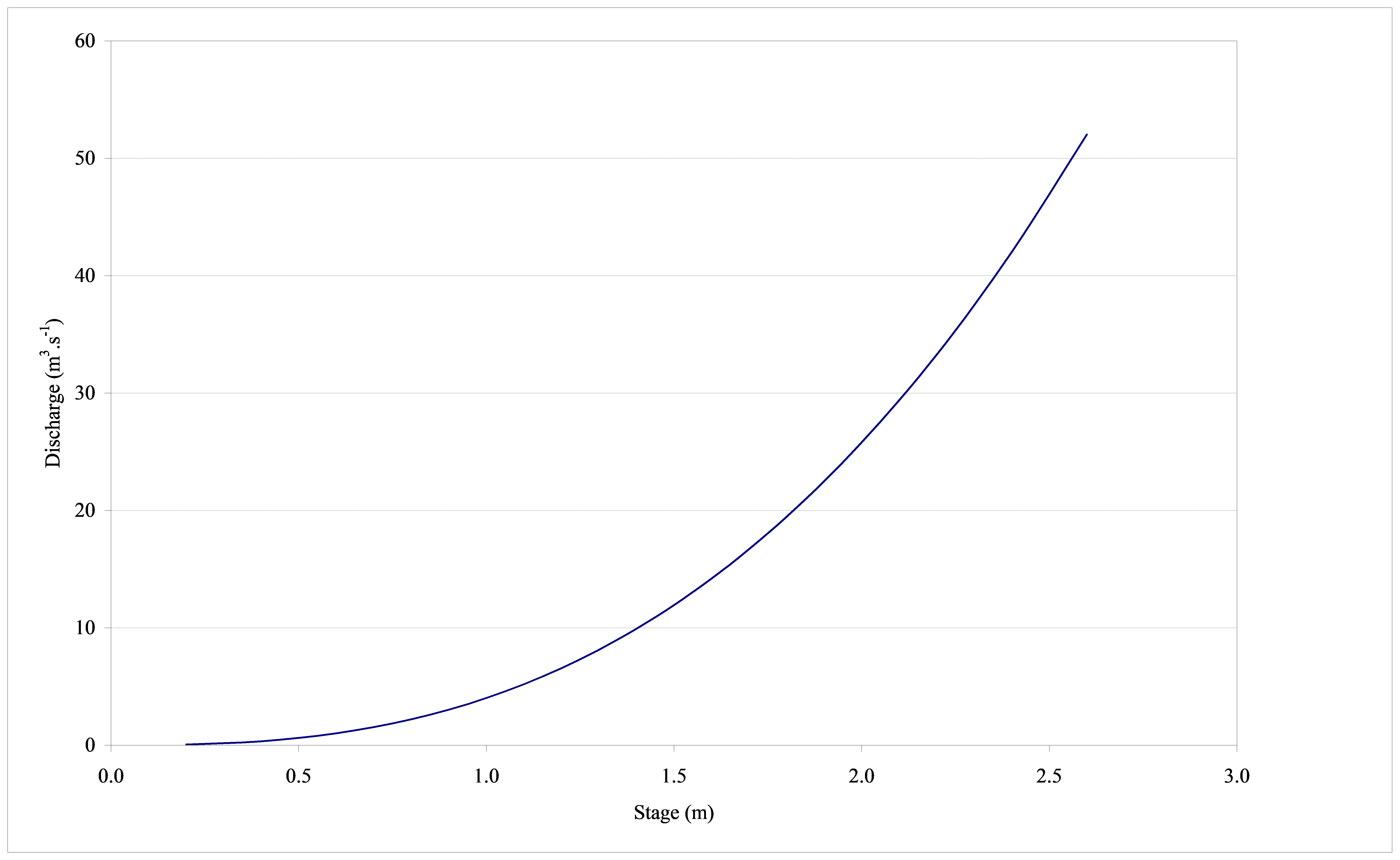
The outflow hydrographs for the selected events were computed using the Muskingum-Cunge method, employing both empirically estimated variables (MC-E) and variables estimated from assumed cross-sections (MC-X). Geometrical parameters of river reaches, including roughness coefficients (n), top flow width (W), cross-section area (A), and wetted perimeter (P), as well as hydraulic parameters such as celerity (V_w), average velocity (V_av), and flow depth (y), were computed based on field observations. Rating curves for the MC-X method, crucial for estimating depths of reference flows (Q₀) in the routing procedure for each of the three reaches, are detailed in Figures 5.12, 5.13, and 5.14, as discussed in Section 3.2.

5.2.1 Reach-I

The estimated catchment characteristics and parameters for Reach-I are contained in Tables 5.13 to 5.16.

Table 5.13 Hydraulic parameters for Reach-I estimated using the MC-E method.

Reach	Event	Vav [m/s]	Vw [m/s]	R [m]	y [m]	S [%]	n
I	1	2.02	2.47	1.13	1.70	0.70	0.045
	2	1.94	2.37	1.07	1.60	0.70	0.045
	3	2.25	2.75	1.33	2.00	0.70	0.045

Table 5.14 Hydraulic parameters for Reach-I estimated using the MC-X method.

Reach	Event	Vav [m/s]	Vw [m/s]	R [m]	y [m]	S [%]	n
I	1	1.78	2.17	0.93	1.40	0.70	0.045
	2	1.69	2.07	0.87	1.30	0.70	0.045
	3	1.82	2.22	0.97	1.45	0.70	0.045

Table 5.15 Estimated parameters for Reach-I using the MC-E method.

Reach	Event	ΔL [m]	Δt [s]	A [m2]	W [m]	Q0 [m3/s]	K [s]	X	C0	C1	C2
I	1	2045	1800	30.31	26.74	61.26	828	0.47	0.96	0.38	-0.34
	2	2045	2520	28.12	26.36	54.58	862	0.47	0.97	0.50	-0.47
	3	4090	1800	29.49	22.12	66.43	1486	0.48	0.97	0.11	-0.08

Table 5.16 Estimated parameters for Reach-I using the MC-X method.

Reach	Event	ΔL [m]	Δt [s]	A [m2]	W [m]	Q0 [m3/s]	K [s]	X	C0	C1	C2
I	1	2045	1800	34.50	39.20	61.26	942	0.47	0.97	0.32	-0.29
	2	2045	2520	32.30	36.40	54.58	990	0.47	0.97	0.44	-0.42
	3	4090	1800	36.54	40.60	66.43	1841	0.49	0.97	0.00	0.02

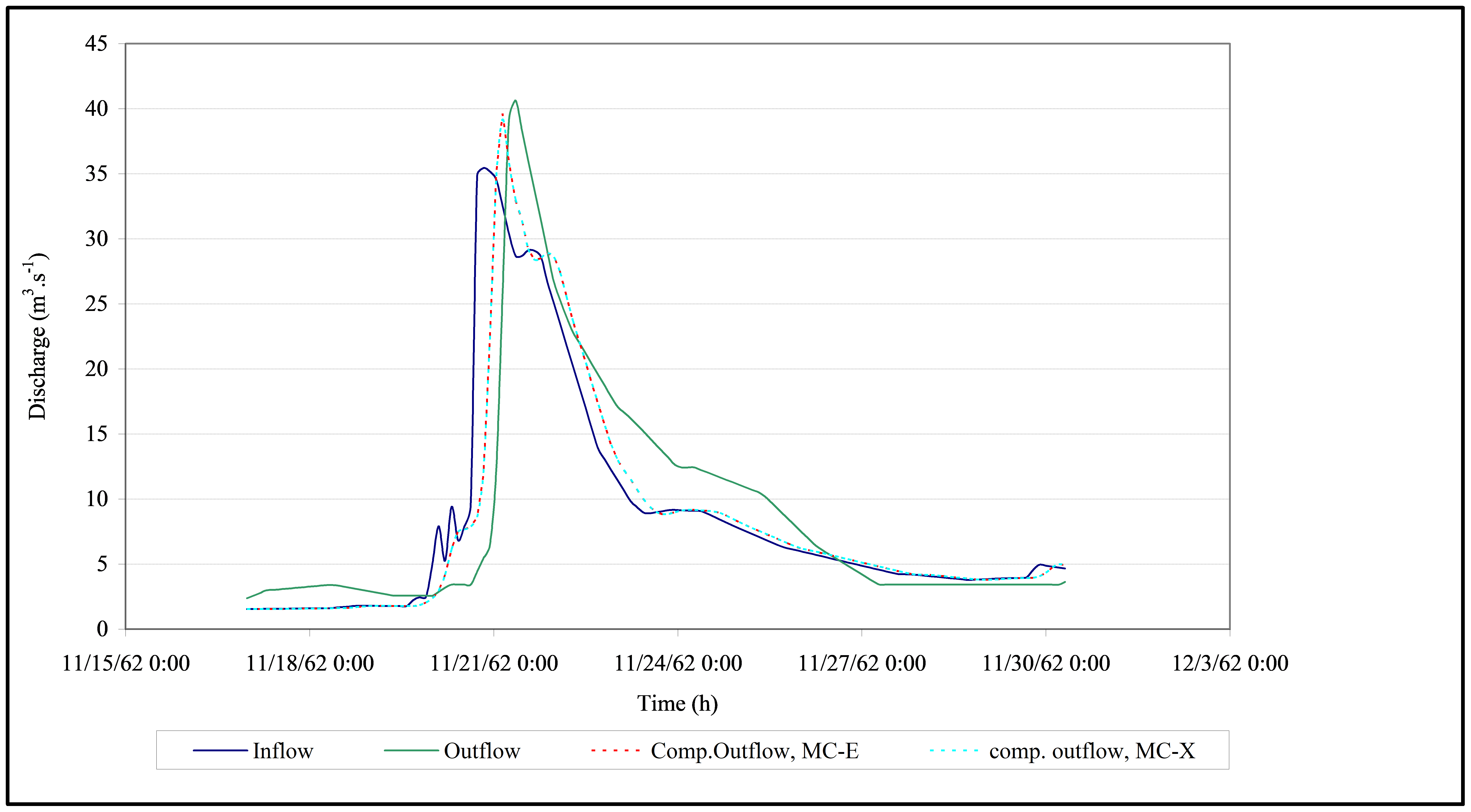
The computed and observed hydrographs from the application of the MC-E and MC-X methods for Reach-I are shown as Figure 5.15 to 5.17.

The results of flood routing analyses using the MC-E and MC-X methods for Reach-I are contained in Tables 5.17 and 5.18.

Table 5.17 Results for Reach-I using the MC-E method.

Reach	Event	Obs Peak Outflow [m3/s]	Comp Peak Outflow [m3/s]	Peak Flow Error [%]	Peak Timing Error [%]	RMSE [m3/s]	Coefficient of efficiency (E)	Obs Volume [million cubic meters]	Comp Volume [million cubic meters]	Volume Error [%]
I	1	105.70	113.05	6.95	-1.59	4.27	0.96	12.63	13.46	6.55
	2	83.67	105.59	26.20	-5.47	7.59	0.88	4.88	5.49	12.59
	3	122.79	129.77	5.68	-5.00	4.27	0.98	10.72	11.01	2.64

Table 5.18 Results for Reach-I using the MC-X method.

Reach	Event	Obs Peak outflow [m3/s]	Comp Peak [m3/s]	Peak flow Error [%]	Peak timing Error [%]	RMSE [m3/s]	Coefficient of efficiency (E)	Obs Volume [million cubic meters]	Comp Volume [million cubic meters]	Volume Error [%]
I	1	105.70	112.98	6.89	-1.59	4.14	0.96	12.63	13.46	6.53
	2	83.67	105.45	26.04	-5.47	7.33	0.89	4.88	5.49	12.58
	3	122.79	129.03	5.08	-5.00	3.92	0.98	10.72	11.00	2.61

The flow depths presented in Table 5.13, derived from empirical relationships, and Table 5.14, derived from an assumed cross-section, exhibit similarity. Consequently, the results from both methods demonstrate similar computed outflow hydrographs. Furthermore, the K and X parameters of both methods are nearly identical, indicating no discernible difference in the computed hydrographs.

Tables 5.17 and 5.18 highlight that Event 2 exhibits a relatively large RMSE error and volume error. However, the statistical results for the other events are generally acceptable and comparable to those obtained using the calibrated methods (M-Cal and M-Ma).

From the result Table 5.18, it is evident that Event 3 has a small RMSE value, a small volume error, and the coefficient of efficiency (E) is nearly equal to one. These results indicate a high degree of correlation between the computed and observed hydrographs. Hence, Event 3 was selected for sensitivity analyses from Reach-I, as detailed in Section 5.3.

5.2.2 Reach-II

The estimated catchment characteristics and parameters for Reach-II are contained in Tables 5.19 to 5.22.

Table 5.19 Hydraulic parameters for Reach-II using the MC-E method.

Reach	Event	Vav [m/s]	Vw [m/s]	R [m]	y [m]	S [%]	n
II	1	1.35	1.66	0.82	1.23	0.55	0.05
	2	1.39	1.70	0.86	1.28	0.55	0.05
	3	1.38	1.69	0.85	1.27	0.55	0.05
	4	1.34	1.64	0.81	1.21	0.55	0.05

Table 5.20 Hydraulic parameters for Reach-II using the MC-X method.

Reach	Event	Vav [m/s]	Vw [m/s]	R [m]	y [m]	S [%]	n
II	1	1.40	1.72	0.87	1.30	0.55	0.05
	2	1.48	1.80	0.93	1.40	0.55	0.05
	3	1.48	1.80	0.93	1.40	0.55	0.05
	4	1.51	1.85	0.97	1.45	0.55	0.05

Table 5.21 Estimated parameters for Reach-II using the MC-E method.

Reach	Event	ΔL [m]	Δt [s]	A [m3]	W [m]	Q0 [m3/s]	K [s]	X	C0	C1	C2
II	1	7777	5400	20.20	24.62	27.32	4698	0.49	0.99	0.08	-0.06
	2	7777	5400	22.58	26.39	31.39	4569	0.49	0.99	0.09	-0.08
	3	7777	5400	21.92	25.91	30.26	4603	0.49	0.99	0.09	-0.07
	4	7777	5400	19.44	24.04	26.04	4743	0.49	0.99	0.07	-0.06

Table 5.22 Estimated parameters for Reach-II using the MC-X method.

Reach	Event	ΔL [m]	Δt [s]	A [m3]	W [m]	Q0 [m3/s]	K [s]	X	C0	C1	C2
II	1	7777	5400	16.90	19.50	27.32	4531	0.49	0.98	0.10	-0.08
	2	7777	5400	19.60	21.00	31.39	4312	0.49	0.98	0.12	-0.10
	3	7777	5400	19.60	21.00	30.26	4312	0.49	0.98	0.12	-0.10
	4	7777	5400	21.03	21.75	26.04	4213	0.49	0.99	0.13	-0.12

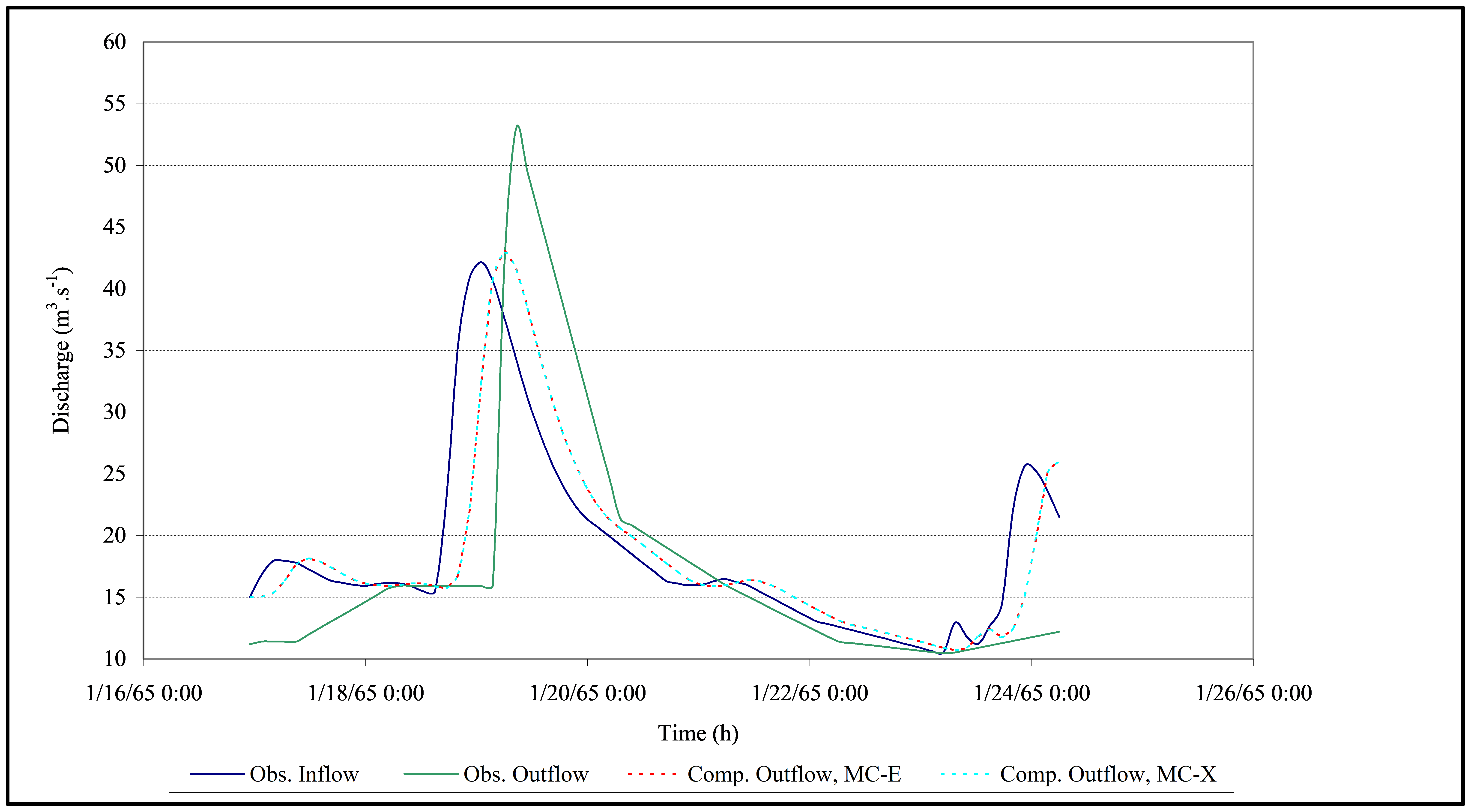
The computed and observed hydrographs from the application of the MC-E and the MC-X methods for Reach-II are shown in Figures 5.18 to 5.21.

The results of flood routing analyses using the MC-E and the MC-X methods for Reach-II are contained in Tables 5.23 and 5.24.

Table 5.23 Results for Reach-II using the MC-E method.

Reach	Event	Obs Peak outflow [m3/s]	Comp Peak [m3/s]	Peak Flow Error [%]	Peak timing Error [%]	RMSE [m3/s]	Coefficient of efficiency (E)	Obs Volume [million cubic meters]	Comp Volume [million cubic meters]	Volume Error [%]
II	1	51.25	47.87	-6.60	1.65	4.52	0.87	13.63	12.36	-9.31
	2	55.52	51.69	-6.90	0.00	7.40	0.82	18.54	20.70	11.68
	3	64.22	57.22	-10.89	0.00	8.98	0.74	19.87	15.62	-21.38
	4	55.40	51.77	-6.55	0.00	2.02	0.97	14.39	13.76	-4.33

Table 5.24 Results for Reach-II using the MC-X method.

Reach	Event	Obs Peak outflow [m3/s]	Comp Peak [m3/s]	Peak flow Error [%]	Peak timing Error [%]	RMSE [m3/s]	Coefficient of efficiency (E)	Obs Volume [million cubic meters]	Comp Volume [million cubic meters]	Volume Error [%]
II	1	51.25	47.65	-7.02	1.65	4.58	0.86	13.63	12.37	-9.20
	2	55.52	51.60	-7.06	0.00	7.51	0.81	18.54	20.64	11.36
	3	64.22	57.14	-11.02	0.00	8.78	0.75	19.87	15.66	-21.17
	4	55.40	51.70	-6.66	0.00	2.07	0.97	14.39	13.77	-4.28

The depth of flow and the Muskingum parameters in both methods are nearly equal, indicating no difference in the computed hydrographs.

As demonstrated in Tables 5.23 and 5.24, Event 4 yielded a relatively small RMSE and large coefficient of efficiency (E) values. Therefore, Event 4 was chosen for sensitivity analysis in Reach-II, as outlined in Section 5.3. The errors for the other events are less than 22% for the statistics considered.

5.2.3 Reach-III

The estimated catchment characteristics and parameters for Reach-III are presented in Tables 5.25 to 5.28.

Table 5.25 Hydraulic parameters for Reach-III using the MC-E method.

Reach	Event	Vav [m/s]	Vw [m/s]	R [m]	y [m]	S [%]	n
III	1	0.85	1.04	1.08	1.62	0.12	0.04
	2	0.91	1.11	1.20	1.80	0.12	0.04
	3	0.88	1.07	1.14	1.71	0.12	0.04
	4	0.78	0.97	0.94	1.42	0.12	0.04

Table 5.26 Hydraulic parameters for Reach-III using the MC-X method.

Reach	Event	Vav [m/s]	Vw [m/s]	R [m]	y [m]	S [%]	n
III	1	0.84	1.03	1.07	1.60	0.12	0.04
	2	0.91	1.11	1.20	1.80	0.12	0.04
	3	0.88	1.07	1.13	1.70	0.12	0.04
	4	0.79	0.96	0.97	1.45	0.12	0.04

Table 5.27 Estimated parameters for Reach-III using the MC-E method.

Reach	Event	ΔL [m]	Δt [s]	A [m2]	W [m]	Q0 [m3/s]	K [s]	X	C0	C1	C2
III	1	4000	9000	21.85	20.25	18.49	3862	0.41	0.90	0.43	-0.33
	2	4000	9000	28.97	24.16	26.31	5998	0.44	0.91	0.24	-0.14
	3	10000	9000	25.15	22.10	22.09	9317	0.46	0.92	0.02	0.05
	4	10000	9000	15.32	16.21	11.89	10547	0.47	0.93	-0.04	0.11

Table 5.28 Estimated parameters for Reach-III using the MC-X method.

Reach	Event	ΔL [m]	Δt [s]	A [m2]	W [m]	Q0 [m3/s]	K [s]	X	C0	C1	C2
III	1	4000	9000	17.07	16.00	18.49	3891	0.38	0.87	0.44	-0.30
	2	4000	9000	21.60	18.00	26.31	5996	0.42	0.88	0.25	-0.13
	3	10000	9000	25.22	17.00	22.09	9343	0.45	0.90	0.03	0.07
	4	10000	9000	15.09	14.50	11.89	10388	0.46	0.93	-0.03	0.11

The computed and observed hydrographs from the application of the MC-E and MC-X methods for Reach-III are depicted in Figures 5.22 to 5.25.

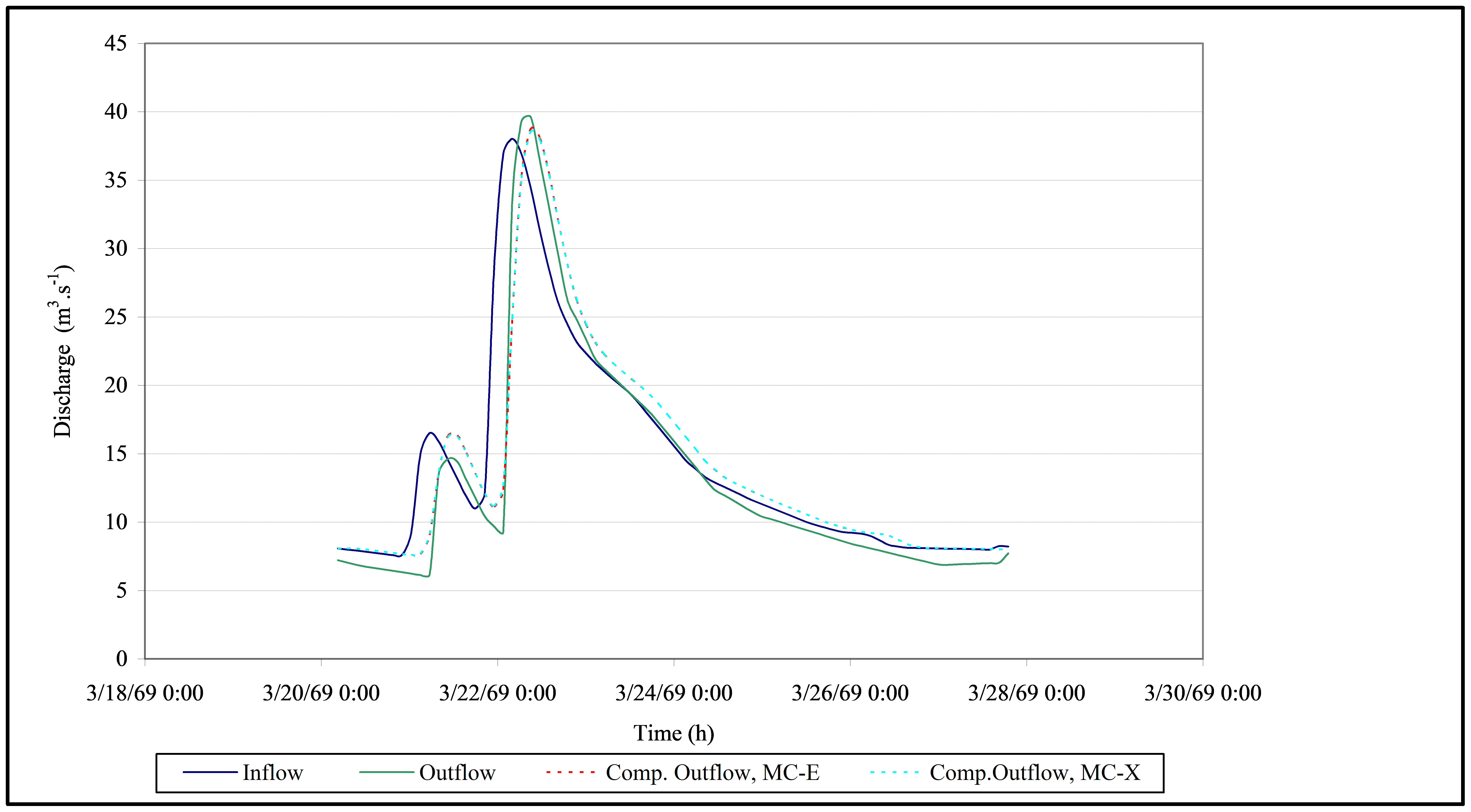
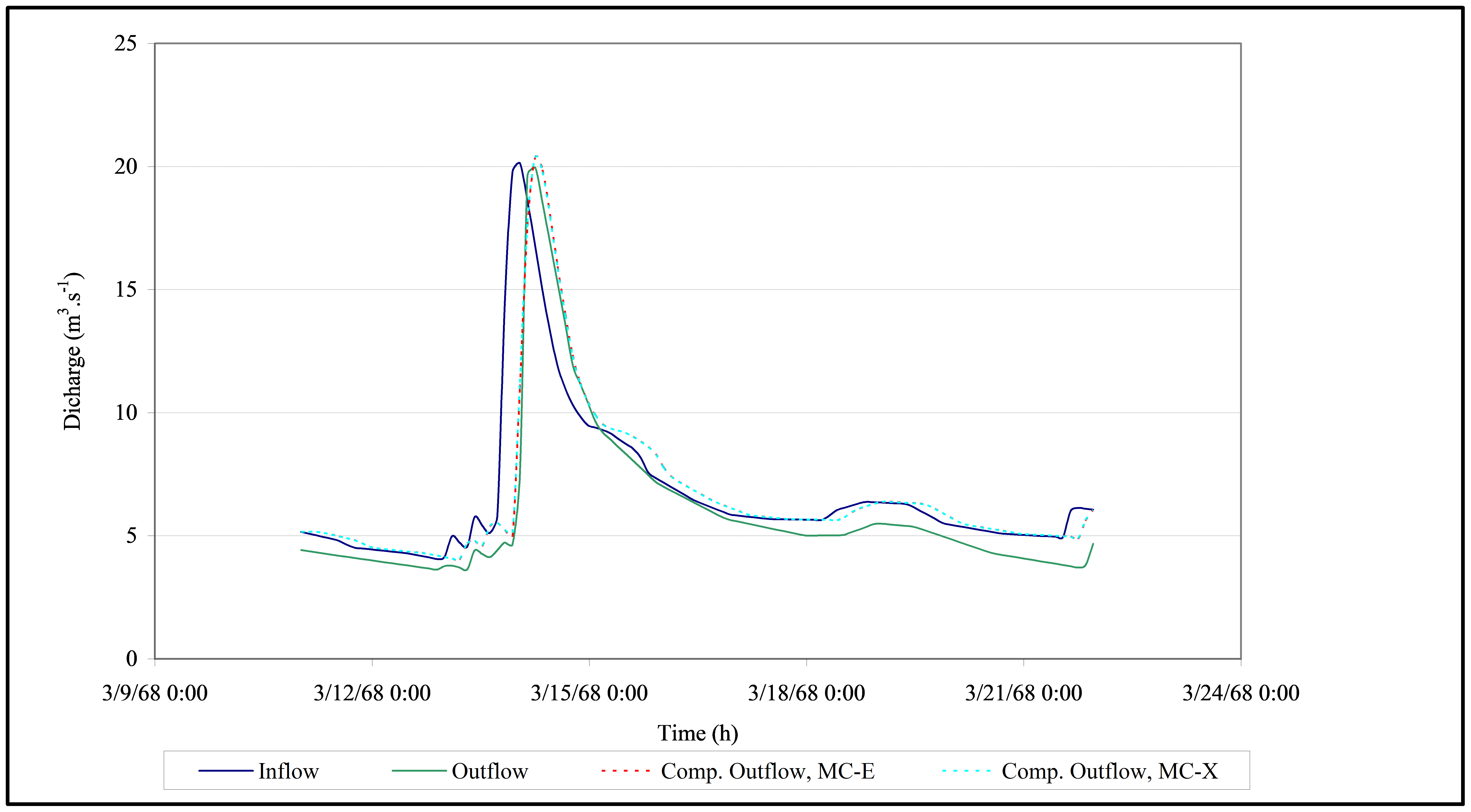
The results of flood routing analyses using the MC-E and the MC-X methods in Reach-III are contained in Tables 5.29 and 5.30.

Table 5.29 Results for Reach-III using the MC-E method.

Reach	Event	Obs Peak outflow [m3/s]	Comp Peak [m3/s]	Peak flow Error [%]	Peak timing Error [%]	RMSE [m3/s]	Coefficient of efficiency (E)	Obs Volume [million cubic meters]	Comp Volume [million cubic meters]	Volume Error [%]
III	1	40.65	39.62	-2.52	2.38	3.70	0.82	10.34	9.71	-6.15
	2	52.97	43.14	-18.55	0.00	5.86	0.64	11.08	11.66	5.28
	3	39.64	38.74	-2.27	0.00	1.77	0.95	8.72	9.45	8.37
	4	19.97	20.36	1.94	0.00	0.88	0.93	5.67	6.36	12.25

Table 5.30 Results for Reach-III using the MC-X method.

Reach	Event	Obs Peak outflow [m3/s]	Comp Peak [m3/s]	Peak flow Error [%]	Peak timing Error [%]	RMSE [m3/s]	Coefficient of efficiency (E)	Obs Volume [million cubic meters]	Comp Volume [million cubic meters]	Volume Error [%]
III	1	40.65	39.20	-3.56	2.38	3.67	0.82	10.34	9.71	-6.15
	2	52.97	42.92	-18.97	0.00	5.85	0.64	11.08	11.66	5.29
	3	39.64	38.53	-2.80	0.00	1.78	0.95	8.72	9.45	8.37
	4	19.97	20.37	1.98	0.00	0.88	0.93	5.67	6.36	12.26

As shown in Tables 5.29 and 5.30 for the MC-E and the MC-X methods, large volume errors were obtained for Event 4. Generally, the results obtained from all of the events show that the computed hydrographs from both methods are similar to the observed hydrographs, with errors of less than 20% for the statistics considered.

Furthermore, Event 3 resulted in relatively small RMSE and large coefficient of efficiency (E) values, as indicated in Tables 5.29 and 5.30. Hence, Event 3 was selected for sensitivity analysis in Reach-III, as shown in Section 5.3.

5.2.4 Section conclusion

As observed in Figures 5.15 to 5.25 and Tables 5.16 to 5.30, the results of computed hydrographs using both empirically estimated parameters and parameters estimated from an assumed cross-section resulted in acceptable results when compared to the observed hydrographs, with errors of less than 26% for the statistics considered. Therefore, it is concluded that the methods can be applied in ungauged catchments.

However, the addition of lateral inflow in the simulated hydrographs was not sufficiently adequate when compared to the observed outflow. As the length of a reach increases, the possibilities of tributary inflows also increase. Hence, in large catchments, the tributary flow should be added separately.

Since the ungauged flood routing methods utilize empirical formulas, the results may not be equal to the calibrated flood routing methods. Nevertheless, the results indicate that the ungauged flood routing methods have estimated the simulated hydrographs with reasonable results when compared to the calibrated method. Therefore, it is concluded that the methods can be applied in situations when there are no observed data sets in the catchments.

From the events analyzed, Event 3 in Reach-I, Event 4 in Reach-II, and Event 3 in Reach-III were selected for sensitivity analyses using the MC-E method.

5.3 Sensitivity Analyses

There are various limitations of the Muskingum-Cunge flood routing method and its assumptions, which were outlined in Sections 2.1 and 2.2. The Muskingum method has different responses to variations in physical catchment parameters such as reach slope, roughness coefficients, and channel geometry used in the model. The statistical analysis of computed hydrographs with the observed hydrographs describes the model performance with regards to specific input variables to the model. Variations in roughness coefficients, reach slope, and channel geometry influence the computed volume, peak flow rate, and timing of the hydrographs. Hence, the sensitivity of the computed hydrographs to a 50% variation of the variables was analyzed. The model sensitivity analyses were undertaken using the three selected events. A 50% variation was used in the sensitivity analysis as this is the typical error that could occur in the estimation of these variables in practice.

The three selected events have a large flow rate with small lag time (Reach-I), medium peak flow rate with large lag time and additional lateral inflows (Reach-II), as well as a small peak flow rate with medium lag time (Reach-III).

Changing the catchment flow variables changes the K and X parameters. Hence, the variation in the outflow hydrographs is due to the change in both the K and X parameters.

5.3.1 Sensitivity analysis for the coefficient of roughness (n)

The values for the roughness coefficient of the river reaches used in this study were subjectively estimated from field observations. The seasonal variation, subjectivity, and other errors may change the estimation of the roughness coefficient, which could influence the simulated hydrographs (Section 2.9.3). To analyze the effect of error in the estimation of the roughness coefficient, hydrographs with a 50% variation in the roughness coefficient were computed for the three events while keeping the other variables constant.

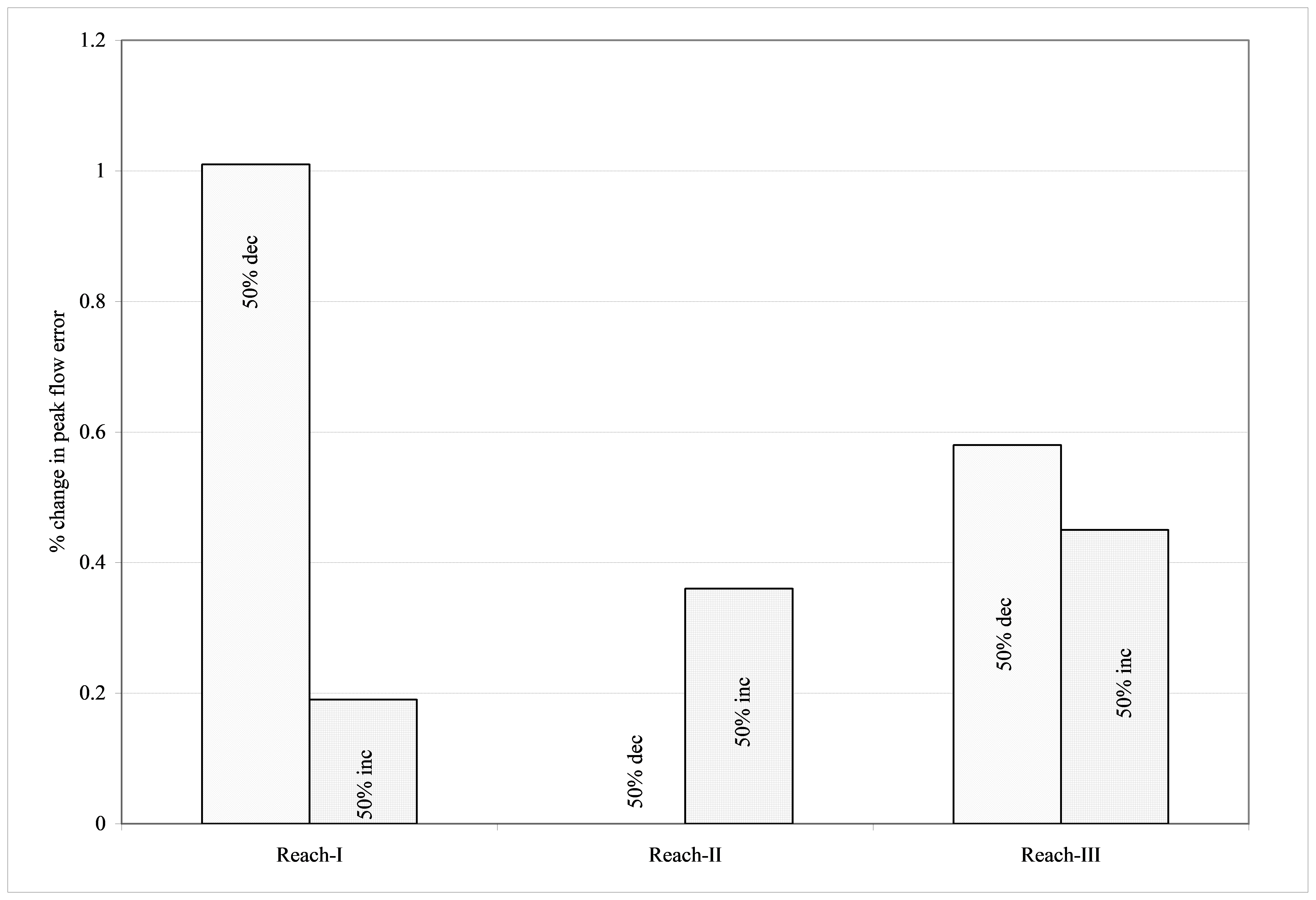
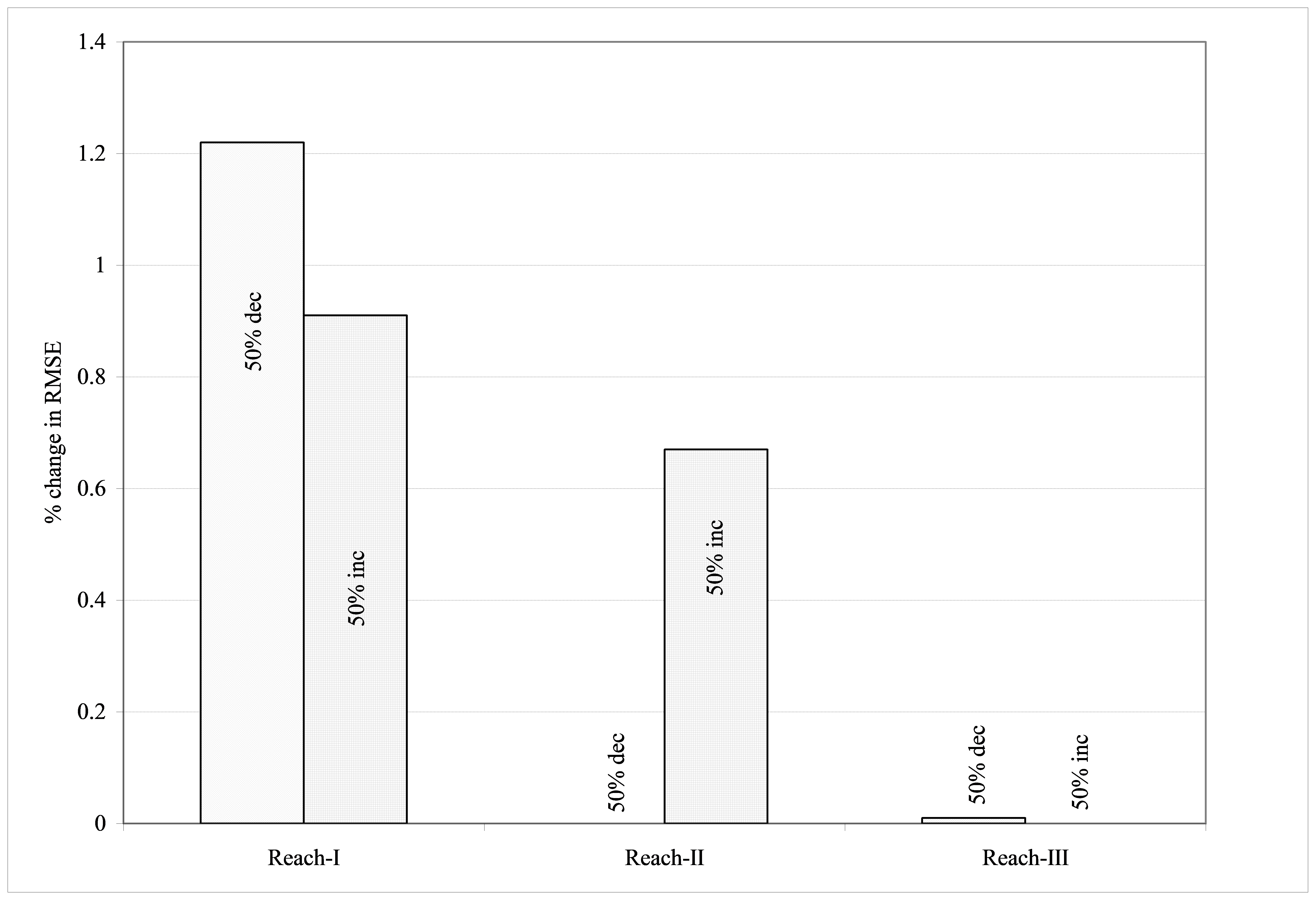
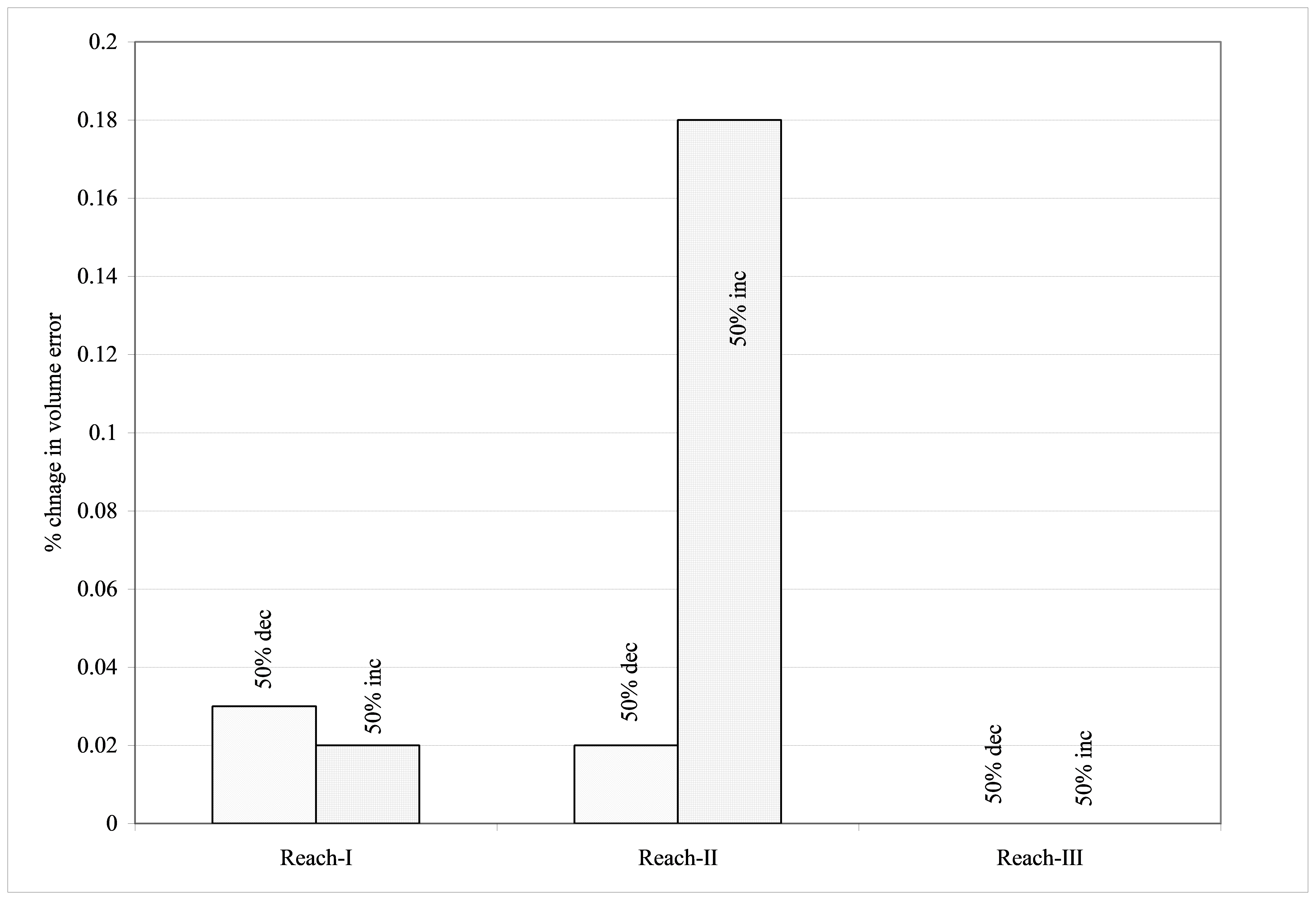
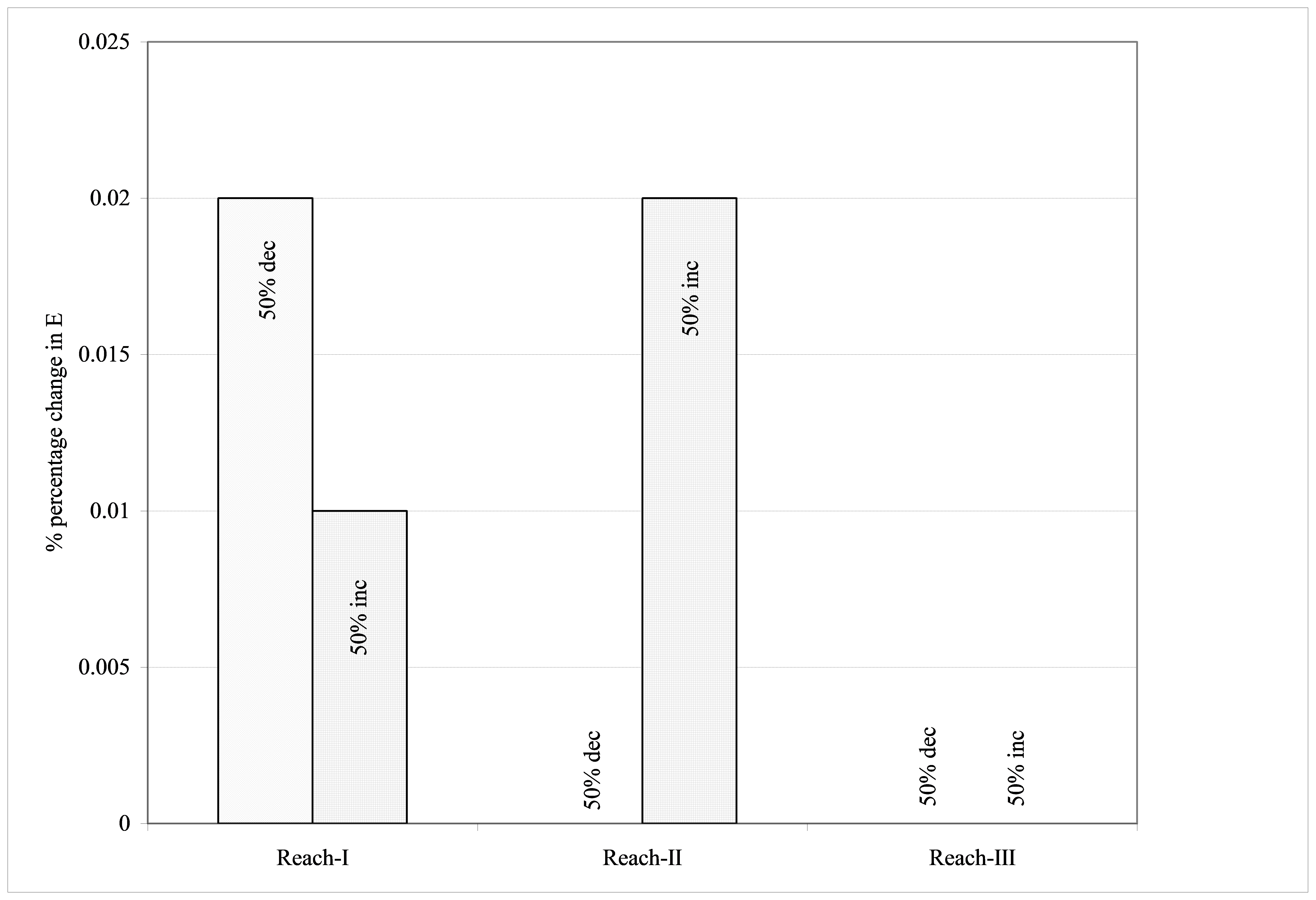
Increasing the roughness coefficient by 50% increases the value of the K parameter and decreases the value of the X parameter. From the results for Reaches-I, II, and III, it is observed that a 50% increase in the roughness coefficient increases the peak error by 0.19%. Decreasing the roughness coefficient by 50% decreases the computed peak error by 1% in Reach-I; increases the peak error by 0.0% in Reach-II, and decreases the peak flow by 0.13% in Reach-III. The variation of response to the same variable change between the reaches may be explained by the fact that the increase or decrease of resistance affects the lower flows more than higher flows. The lateral inflow into the main reach may also have an effect on the variation of roughness coefficients in Reach-II and Reach-III.

Figures 5.26 to 5.29 show the effect of variation of roughness coefficient on peak flow, shape, and volume of hydrographs for the selected three events.

From the results obtained, it is evident that the performance of the MC-E method is insensitive to the value of the roughness coefficient used, i.e., a 50% variation in the roughness coefficient resulted in a change of less than 1% error for all the performance statistics considered.

5.3.2 Sensitivity Analysis for the Slope (S)

The sensitivity analysis indicates that altering the slope parameter has distinct effects on the K and X parameters. An increase in slope leads to a decrease in the K parameter and an increase in the X parameter.

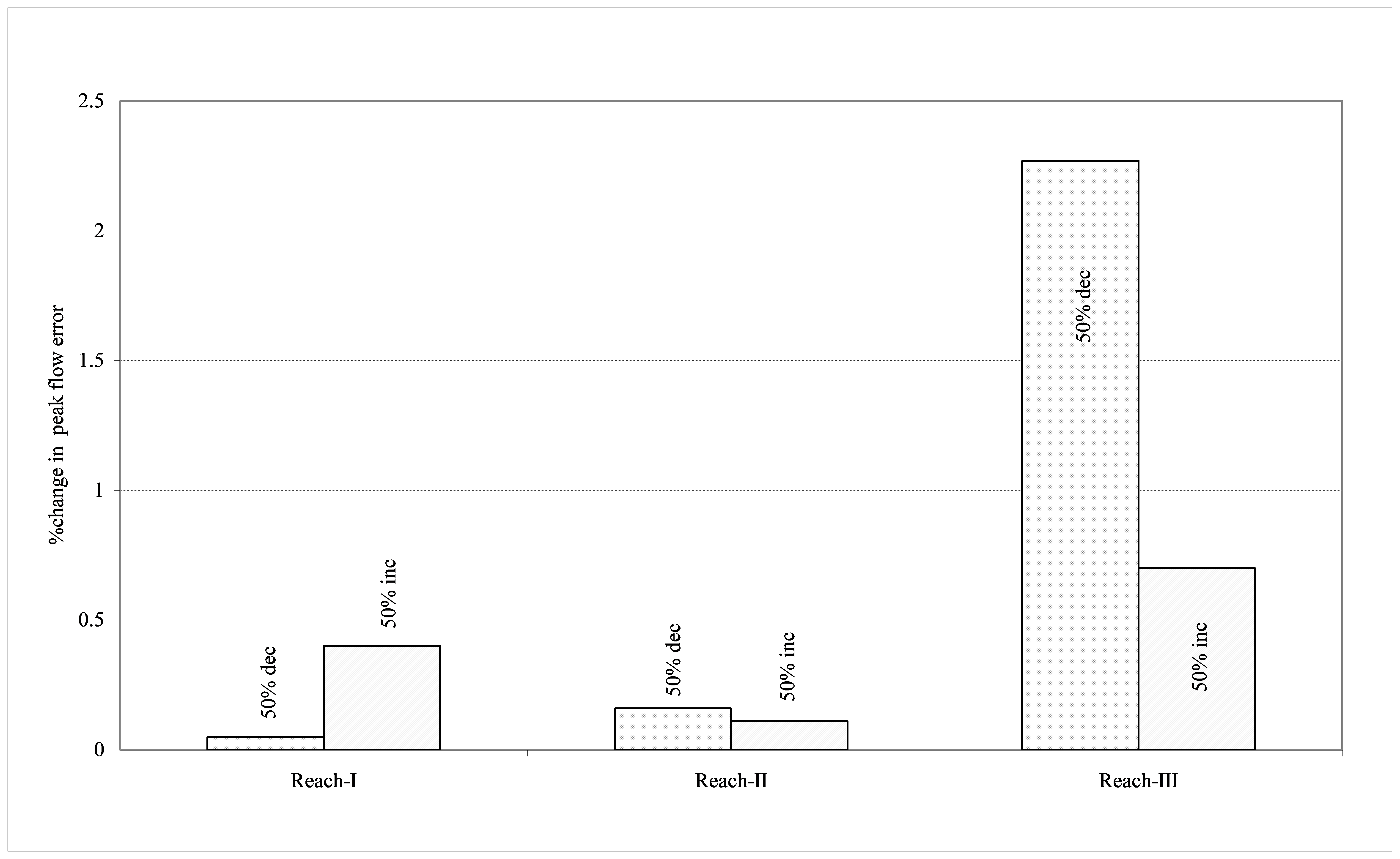
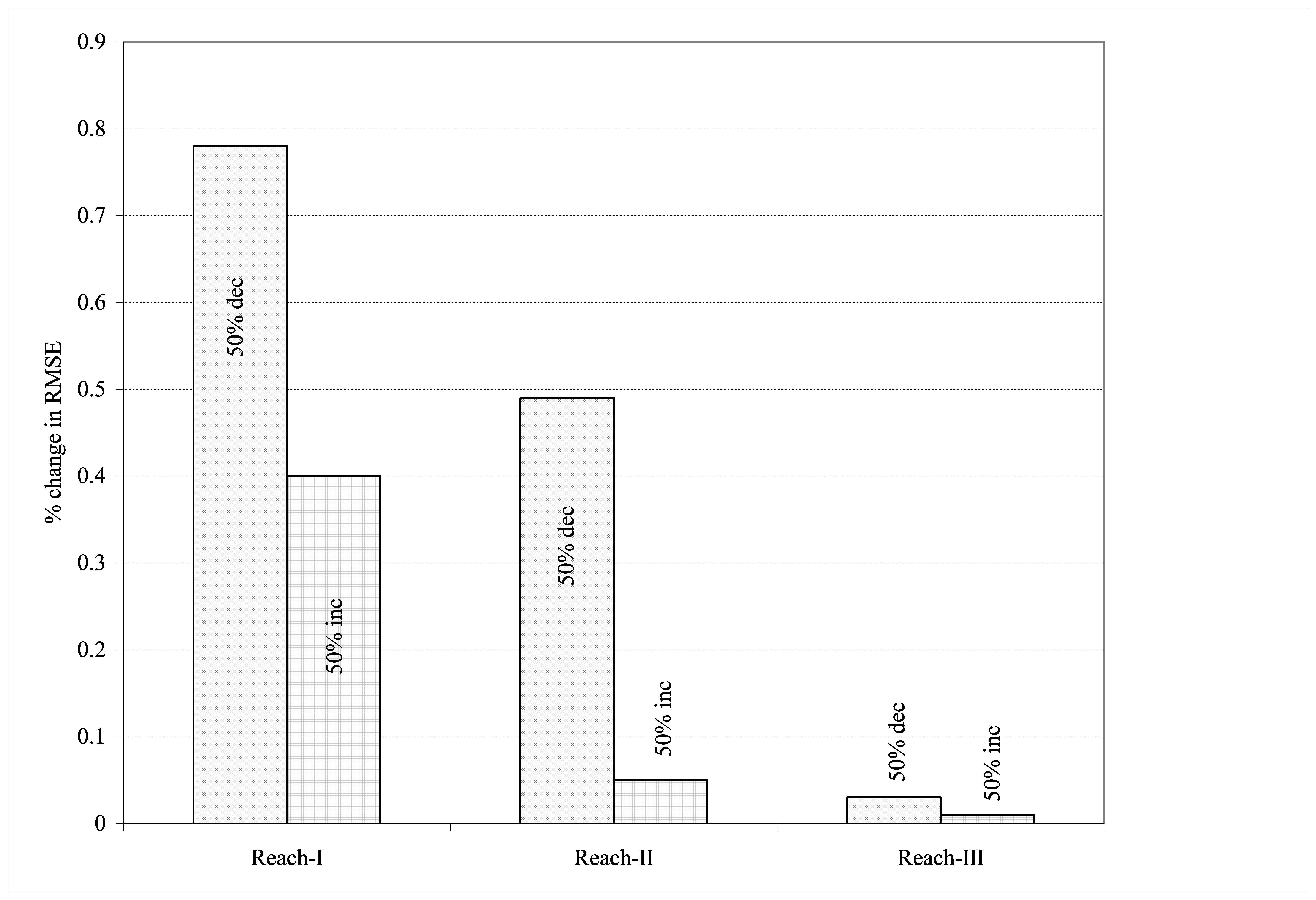
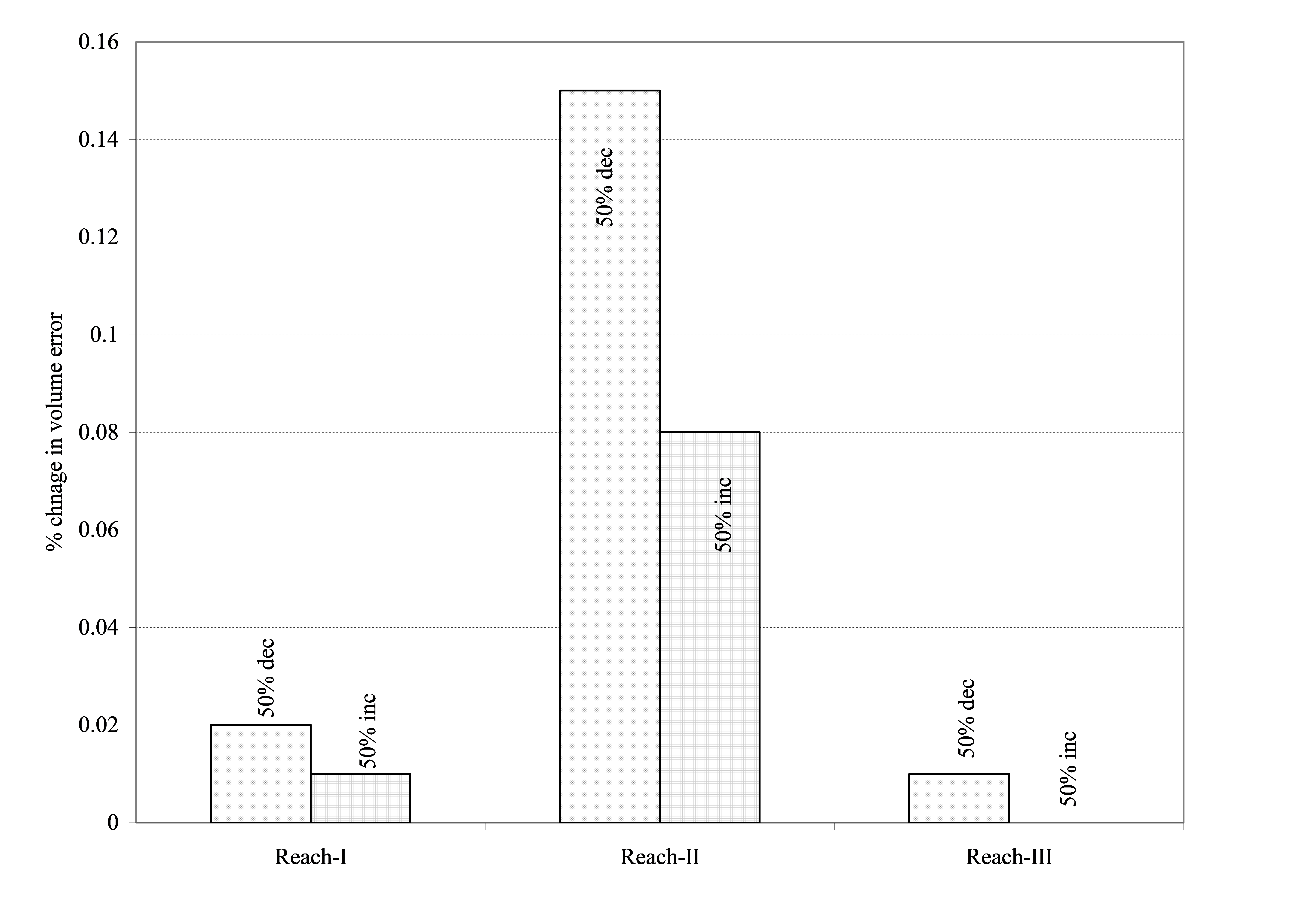
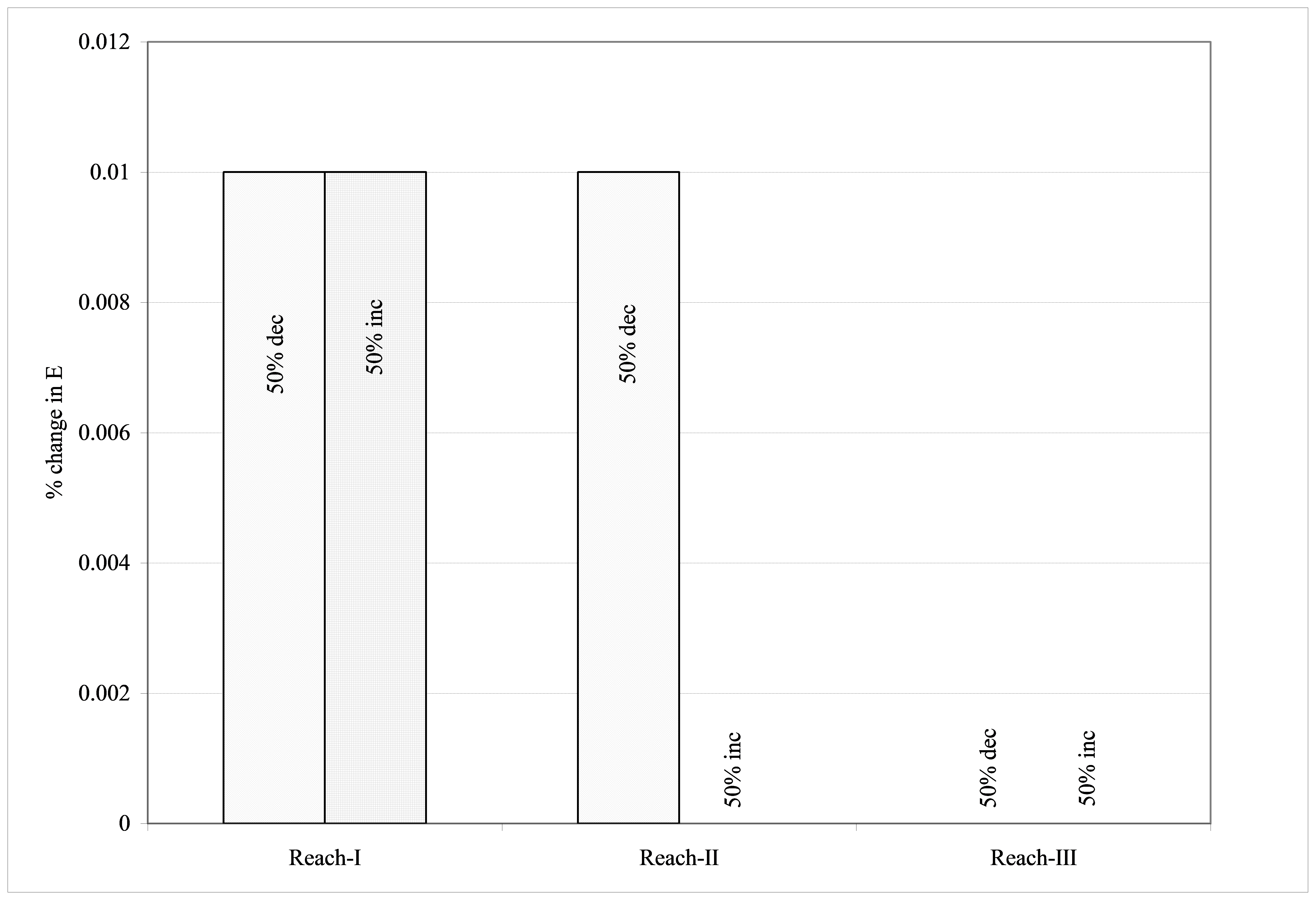
Figures 5.30 to 5.33 depict how variations in reach slope impact the peak flow, shape, and volume of hydrographs for the three selected events. Generally, an increase in slope results in higher flow velocities, leading to a reduction in lag time and an apparent increase in peak discharge magnitude.

Analysis of slope variations by 50% reveals that the relative error in all considered performance statistics remains below 2%. Therefore, a 50% variation in slope has minimal impact on the routing process.

5.3.3 Sensitivity Analysis for Channel Geometry

Changing the geometry of the channel section is expected to affect both the K and X parameters. As shown in Table 4.1 (Section 4), the ratio of kinematic wave velocity (celerity) to average velocity for wide rectangular channels is larger than for triangular and parabolic section channels. The ratio of celerity to velocity for a triangular section is larger than that for a parabolic section channel. From the sensitivity analysis, it was observed that the changes in peak flow errors are lowest for a triangular section. Figures 5.34 to 5.37 show the effect of variation in channel geometry from a parabolic section on changes in peak flow, shape, and volume of hydrographs for the selected three events.

The sensitivity of flow to channel geometry shows that there is a decrease in RMSE and an increase in the coefficients of efficiency (E) when there is a change in geometry from rectangular to parabolic and to triangular sections.

These results show that different assumed geometrical shapes have an effect on the computed hydrographs. However, the performance statistics vary by less than 1%, and hence it is concluded that the selection of cross-sectional shape is not important for flood routing using the MC-E method.